the Creative Commons Attribution 4.0 License.
the Creative Commons Attribution 4.0 License.
 | 09 Sep 2019
Electrical formation factor of clean sand from laboratory measurements and digital rock physics
Mohammed Ali Garba
Stephanie Vialle
Mahyar Madadi
Boris Gurevich
Maxim Lebedev
Electrical properties of rocks are important parameters for well-log and reservoir interpretation. Laboratory measurements of such properties are time-consuming, difficult, and impossible in some cases. Being able to compute them from 3-D images of small samples will allow for the generation of a massive amount of data in a short time, opening new avenues in applied and fundamental science. To become a reliable method, the accuracy of this technology needs to be tested. In this study, we developed a comprehensive and robust workflow with clean sand from two beaches. Electrical conductivities at 1 kHz were first carefully measured in the laboratory. A range of porosities spanning from a minimum of 0.26–0.33 to a maximum of 0.39–0.44, depending on the samples, was obtained. Such a range was achieved by compacting the samples in a way that reproduces the natural packing of sand. Characteristic electrical formation factor versus porosity relationships were then obtained for each sand type. 3-D microcomputed tomography images of each sand sample from the experimental sand pack were acquired at different resolutions. Image processing was done using a global thresholding method and up to 96 subsamples of sizes from 2003 to 7003 voxels. After segmentation, the images were used to compute the effective electrical conductivity of the sub-cubes using finite-element electrostatic modelling. For the samples, a good agreement between laboratory measurements and computation from digital cores was found if a sub-cube size representative elemental volume (REV) was reached that is between 1300 and 1820 µm3, which, with an average grain size of 160 µm, is between 8 and 11 grains. Computed digital rock images of the clean sands have opened a way forward for obtaining the formation factor within the shortest possible time; laboratory calculations take 5 to 35 d as in the case of clean and shaly sands, respectively, whereas digital rock physics computation takes just 3 to 5 h.
- Article
(3034 KB) - Full-text XML
- BibTeX
- EndNote


Electrical formation factor (FF) refers to the ratio of the electrical resistivity of a saturated medium (sediment or rock) to that of the saturating fluid (Guéguen and Palciauskas, 1994). This is an important parameter in exploration geophysics as, contrary to the electrical resistivity of reservoirs that is dependent on the resistivity of the saturating fluid (and hence the same type of reservoir can exhibit high or low resistivities; Constable and Srnka, 2007; Jinguuji et al., 2007; Mitsuhata et al., 2006), the formation factor is an intrinsic property of the rock independent of fluid salinity. Measurement of the formation factor in the laboratory is often difficult and time-consuming, if not impossible in some cases. Minerals forming the rock or sediment sample must reach thermodynamical and electrical equilibrium with the saturating fluid, which typically takes 4 to 6 d in a high-permeability, high-porosity clean sandstone but may require at least 4 to 6 weeks for a tight gas sand or a low-porosity rock or sediment with a high clay content. Furthermore, results are affected by current leakage problems (especially at high frequencies) and electrode polarization (emphasized at low frequencies).
Hence, the computation of electrical properties from microstructural models has been investigated by several teams in the past 50 years. Various methods have been proposed, from statistical models used to reconstruct 3-D porous materials (e.g. Miller, 1969; Joshi, 1974; Milton, 1982; Torquato, 1987; Adler et al., 1990, 1992; Yeong and Torquato, 1998) to direct measurement of a 3-D structure from synchrotron and X-ray computed microtomography (XRCM) (e.g. Dunsmuir et al., 1991; Spanne et al., 1994; Arns et al., 2001; Øren and Bakke, 2002; Nakashima and Nakano, 2011; Øren et al., 2007) or laser confocal microscopy (Fredrich et al., 1995). In most of these studies using XRCM images, the numerical prediction of electrical conductivity underestimates the experimental results by 30 % to 100 % (which leads to an overestimation of the formation factor) (Spanne et al., 1994; Schwartz et al., 1994; Auzerais et al., 1996). Several explanations have been put forward to justify such a discrepancy: percolation differences between the model and real material, mainly due to smaller volume sampling in the model (Adler et al., 1992; Bentz and Martys, 1994); the addition of a third phase to the traditional two-phase model (the rock matrix being one phase and the saturating fluid being a second phase) that counts for the bound fluid at the grain fluid interface (Zhan and Toksoz, 2007); and discretization errors and statistical fluctuations (Arns et al., 2001).
The underlying question behind the computation of electrical properties of digital porous media samples (or any other rock or transport properties) is whether the obtained numerical values are accurate. One aspect of this question relates to the technology itself, namely 3-D imaging, image processing and segmentation, and the suitability and stability of the numerical code. These three key elements of the technology have been investigated by various teams, and the most comprehensive and exhaustive study performed on the various steps of the digital rock physics workflow is the benchmark comparison from Andrä et al. (2013a, b). As they are using various rock types and processing and computing methods, the comparison is complex: they concluded that the computed effective rock properties are affected by segmentation processes, the choice of digital sub-volume, and the choice of numerical code and boundary conditions. Nonetheless, the different values obtained for the formation factor deviated at most by 23 % from the midrange value (Andrä et al., 2013a). For the sphere pack sample, all computed formation factors ranged from 4.3 to 4.8.
The second aspect of this question relates to the comparison of the computed values with laboratory-scale experimental data to validate the correctness of the digital rock physics workflow. However, because both experiments are done at a different scale (centimetre scale for the laboratory and millimetre scale for the digital computation) and because rocks are heterogeneous at all scales, the laboratory-measured and digitally computed values do not have to match. Instead, trends between two properties (e.g. formation factor and porosity) computationally derived and produced in the laboratory should be in good agreement (Dvorkin et al., 2011; Andrä et al., 2013a).
In the work described in this paper, we propose a robust workflow to digitally compute the electrical properties of clean (i.e. that does not contain any clay or other conductive minerals) unconsolidated porous media. We first carefully measure in the laboratory the formation factor of two beach sand samples of similar mineralogy (quartz and carbonate), but of different grain size, over a wide range of porosities obtained by compacting the sand sample. Hence, trends in formation factor versus porosity that reproduce a packing as close as possible to the one found in situ were obtained. We then compute the formation factor from X-ray microtomography images using the free software and finite-element electrostatic code from the National Institute of Standards and Technology (NIST) with multiple subsamples of various sizes. To our knowledge, this is the first time that such work has been done on clean sand.
2.1 Sample collection and preparation
The samples investigated in this paper are sand samples collected from the coastal margin of the Perth Basin, Western Australia. The Perth Basin is an elongate, north–south-trending trough underlying approximately 100 000 km2 of the Western Australian margin. Sediments were shed from the adjacent Yilgarn block. The Yarragadee and Leederville sandstone formations are intercalated with the Tamale limestone that forms the carbonates at the Upper Cretaceous. One sample was collected from Scarborough Beach (31∘53′41.97 S, 115∘45′17.74 E) and one from Cottesloe Beach (31∘59′40.62 S, 115∘45′03.70 E). All the samples are composed of quartz and carbonate in 80 % / 20 % (volume) proportion, respectively, as determined from the three-phase watershed segmentation presented in Sect. 3.2.2 of this paper. Grain size was determined by micro-CT image analysis and is between 16 and 794 µm (median 140 µm) for quartz grains and between 19 and 446 µm (median 168 µm) for carbonate grains at Scarborough Beach. It is between 17 and 606 µm (median 159 µm) for quartz and between 15 and 415 µm (median 172 µm) for carbonate grains at Cottesloe Beach. Sand samples were thoroughly washed clean with tap water to remove any plants and grass debris. Loose moist sand was then packed into the different cells used to perform the electrical resistivity measurements, forming an initially high-porosity loose random pack; decreasing porosity in subsequent experiments was achieved by shaking the cell and using tied sticks to compact the sand. This was done in a way to achieve a packing as close as possible to the one found in situ. A range of six different porosities was obtained for the Scarborough Beach sand samples, with an initial porosity of 0.40 (loosely packed) down to 0.27 when highly packed, while five and four different porosities were obtained for the Cottesloe Beach sand, depending on the geometry of the cell, with the loosely packed sample having a porosity of 0.39 and the highly packed sample having a porosity of 0.30.
Porosity was determined from the weights and densities of the sand grains and the known volumes of cells used in the experiment as
where ϕ is porosity, Vt is the total volume of the cell, m is the average mass of the dry sand before and after the experiment, and ρ is the density of the sand grains. Grain density was measured by He pycnometry and found to be equal to 2.71 g cm−2.
2.2 Laboratory set-up and measurements
2.2.1 Experimental set-up
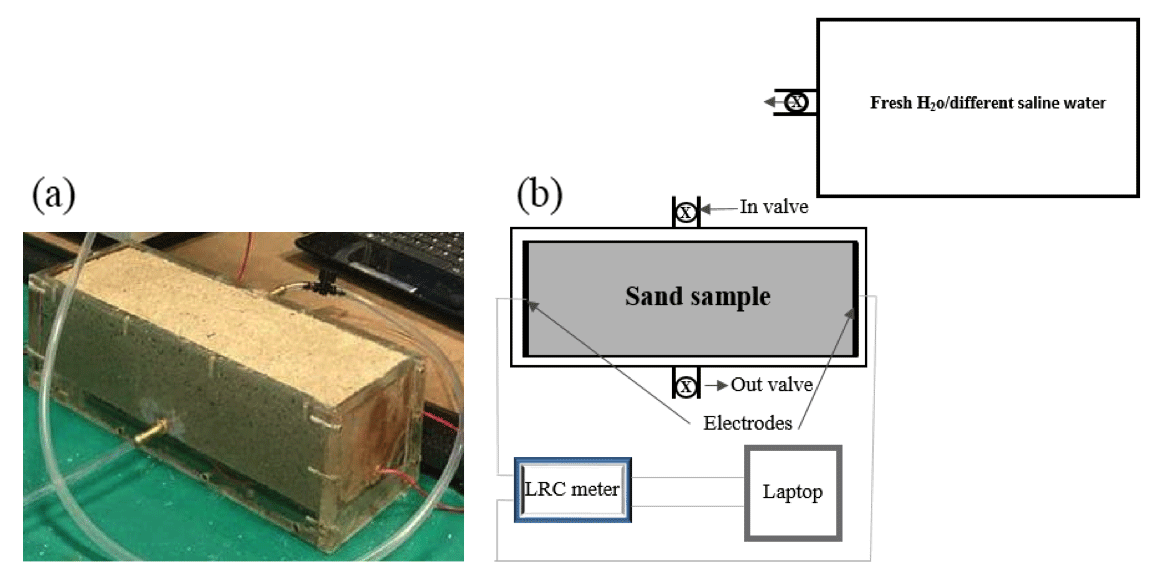
Two different types of cells are used in the experimental set-ups, which were utilized to monitor the electrical resistivities of the sand samples as a function of the salinity of the saturating pore water. The two experimental set-ups are outlined in Figs. 1 and 2. For the cell called the “flow cell”, the sample electrical resistances are measured, while saline solutions of increasing salinities are continuously flooded through the sand samples. Before proceeding with the next saline solution, the reading of the sample's electrical resistance is left to stabilize for a few hours. For the cell called the “static cell”, the sand samples are successively saturated with saline solutions of increasing salinities, left to equilibrate with no fluid flow until stability of the sample electrical resistance reading is achieved, and then drained before saturating the sand sample with the next saline solution. Thus, the utilization of this cylindrical-shaped static cell drastically reduces the experimental time; however, the sample preparation for the static cell is easier than for the flow cell. The flow cell is of cylindrical shape, 27 cm in length, and 5 cm in radius (total volume of 2120.6 cm3), while the static cell is of rectangular shape, 29.8 cm in length, 8.7 cm in width, and 6.2 cm in height (total volume of 1607.41 cm3).

Both cells are made up of Perspex (acrylic) and have an outlet and an inlet connected by tubing to a tank that serves as a reservoir for the various solutions injected into the sand samples. The solutions flow through the sand samples via gravity (falling-head method) and, for the flow cell, two valves at the inlet and outlet are used to achieve a flow rate ranging from 0.52 to 2.75 mL s−1. This flow rate is continuously recorded.
Injected solutions are fresh and saline solutions made with tap water and table salt in various amounts: five different salinities of 0, 5, 15, 25, and 35 g L−1 were achieved and measured on an electric balance (Napco JA-5000), and the solution was stirred until complete dissolution of the salt into the water.
Both cells are equipped with two electrodes made of zinc wire gauze with surface areas of 78.55 and 53.94 cm2 for the dynamic and static cells, respectively. The electrodes are glued at the bottom and at the lid cover of the cylindrical dynamic cell, while they are fixed on both sides of the rectangular static cell; the two electrodes of each cell are connected to an LCR meter (Stanford Research Systems SR720) connected to a laptop to monitor the electrical resistance of the sand sample. The recording time interval for the dynamic cell laboratory measurements is taken at 1 min, while the recording time interval for the static cell laboratory measurement is 10 min. A drive voltage of 1 Vrms is applied and a frequency of 1 kHz is chosen to minimize the phase angle between the voltage and current (i.e. electrode polarization). With these conditions, the monitored Q factor did not exceed 0.095, indicating that the system is nearly purely resistive. For the dynamic cell laboratory measurements, the conductivity of the injected solutions coming out of the cell is monitored by an encased conductivity meter (Hanna edge) attached to the cell at intervals of 1 min to make it synchronous with the sand sample resistance measurements. The fluid electrical conductivity for the static cell set-up is measured with the same probe using the saturating solution drained from the sand sample once the resistance has become stable.
2.2.2 Computation of electrical formation factor
Because the sand samples do not contain any clay and because the injected solutions have a conductivity (10−2 to S m−1) much larger than that of quartz or carbonate surface conductivity ( S m−1 following Miller et al., 1988, and S m−1 following Vialle, 2008), surface and matrix electrical conductivities can be neglected (e.g. Johnson and Sen, 1988; Garrouch and Sharma, 1994). The electrical formation factor F is then given by
with
where Rs is the resistivity of the sand sample saturated with water, Rw is the resistivity of the water, rs the measured resistance of the sand sample saturated with water, A the surface area of the electrode, L the length of the cell, and σw the measured conductivity of water.
To obtain the formation factor, the sample's resistivity, once it has stabilized, is plotted against the saline water's resistivity, and the formation factor is given by the inverse of the slope. Such a plot is given in Fig. 3 for the example of a Cottesloe Beach sample with porosity 33 %.
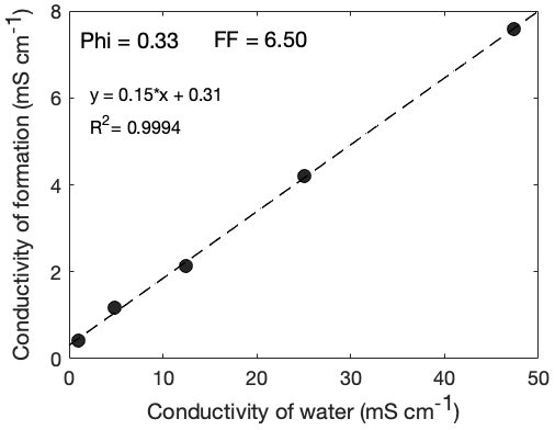
Figure 3Sand sample conductivity as a function of water conductivity for the Cottesloe Beach sample with a porosity of 33 %. The slope of the linear correlation gives a formation factor (FF) of 6.50.
3.1 Image acquisition
Two samples were prepared for imaging with X-ray microcomputed tomography (XRMCT): one from Scarborough Beach and one from Cottesloe Beach. Loose sand was put in a cylindrical Pyrex glass tube of 6 mm diameter and 6 cm height, and the tube was inserted into the core holder of the microtomograph. The samples were scanned with the 3-D X-ray microscope Versa XRM 500 (Zeiss–XRadia) using an X-ray energy of 60 keV, a current of 70.66 mA, and a power of 5 W. In each scan 3000 projections (radiographs) were acquired. The exposure time was 2 s per radiograph. Initial cone-beam 3-D image reconstruction was performed using the software XM Reconstruction (XRadia). A secondary reference was required to remove geometrical artefacts during reconstruction. After 3-D reconstruction, 3-D volume was sliced onto 2-D images for further processing. A total of 1021 2-D images for the Scarborough Beach sample and 991 2-D images for the Cottesloe Beach sample were available for analysis. Total scanning time was 2 h 55 min and 2 h 42 min for the Scarborough and Cottesloe samples, respectively. Nominal voxel sizes of 2.5761 and 2.5516 µm3 were achieved with source-to-sample and detector-to-sample distances of 11 and 22 mm, respectively, for the Scarborough and Cottesloe Beach samples.
3.2 Image processing
3.2.1 Image filtering
We used the software package Avizo Fire 9 (FEI Visualization Sciences Group) for image enhancement and segmentation. Greyscale images of the 2-D slices were processed using a non-local means filter in the intensity range of 255–5344 for Scarborough Beach and 255–5467 for Cottesloe Beach, with the aim of removing ring artefacts in the images and properly enhancing interfaces between the pores and grains as well as removing noise. A non-local means filter has been shown to effectively remove ring artefacts without introducing edge smoothing, in contrast to many other filters, and thus does not require the use of an additional mask (see, for example, the review paper of Schlüter et al., 2014).
Figure 4a–d show raw and filtered images for both Scarborough and Cottesloe Beach: we can easily notice that the quality of the image has increased. In these images, the white grains are carbonate, grey grains are quartz, and black within the disc corresponds to void space (pores).

Figure 4(a) Raw and (b) filtered images of the Scarborough Beach sand sample; (c) raw and (d) filtered images of the Cottesloe Beach sand sample.
3.2.2 Image segmentation
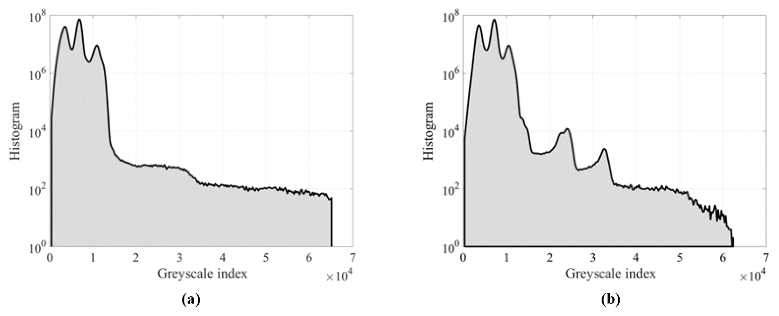
The filtered images were segmented using two types of thresholding algorithms: the first one resulted in a two-phase segmentation that was further used for computing sample electrical conductivities; the second one was a watershed algorithm that resulted in a two- or three-phase segmentation used for grain analysis. Note that filtering and segmentation workflows were applied to the full 3-D dataset. Figure 5 shows the histogram for both samples.
Two-phase segmentation by global thresholding
Because both quartz and carbonate have very low conductivity compared to water, they can be both considered non-conductive for computation purposes of the electrical conductivity of the water-saturated sand sample. Hence, quartz and carbonate can be put in a single phase, and pores will constitute a second phase that will later be filled with a conductive fluid for the computation of sample electrical properties. We use a global threshold segmentation algorithm to separate pores from grains: the set intensity value separating pores from grains (both quartz and carbonate grains having higher intensity values than pores) is kept the same for all 2-D slices.
Poor segmentation can affect the accurate calculation of porosity. To check the quality of the segmentation, we compare the porosity estimated in the laboratory with the one estimated from micro-CT scan images. We made a random loose pack of sand (cm3) in the laboratory to obtain the highest porosities of 0.361 and 0.349 from Scarborough and Cottesloe beaches, respectively, while the smaller scanned sample of the sand (mm3) was also randomly packed in the small tube, from which porosities of 0.369 and 0.359 were obtained from the images of Scarborough and Cottesloe beaches, respectively.
Watershed segmentation
We used a marker-based watershed segmentation algorithm from Avizo Fire 9. We defined either two or three marker ranges of greyscale intensity: for pores and grains or for pores, carbonate grains, and quartz grains. We then performed a watershed flooding for each of these two or three phases. The two-phase watershed segmentation allows for the computation of pore volume and grain size distribution, whereas the three-phase segmentation (Fig. 6) gives the volume fraction of the different minerals.
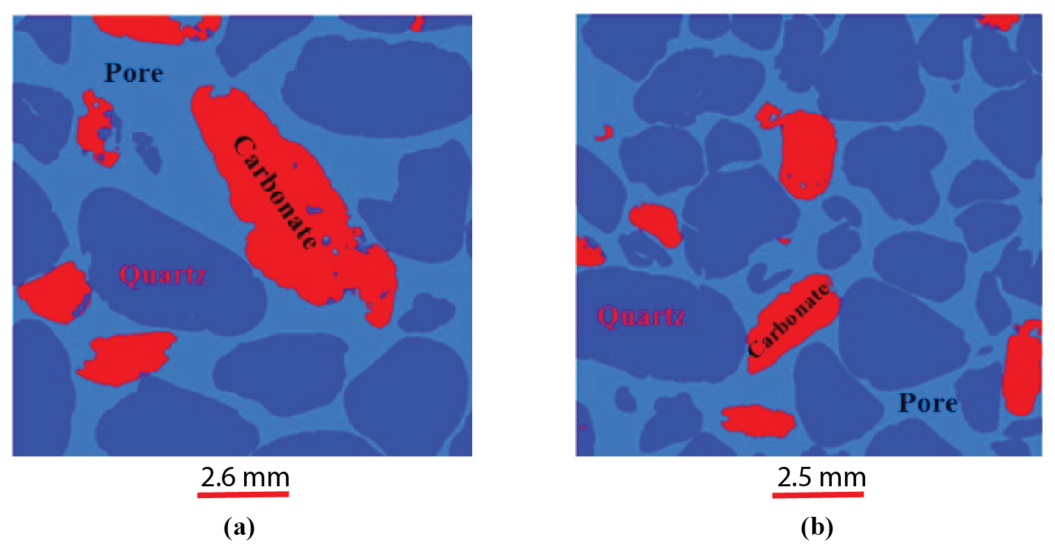
Figure 6Three-phase watershed segmentation of the sand samples: (a) Scarborough; (b) Cottesloe.
From this segmentation, we computed the volume fraction of quartz and carbonate (excluding the pore volume). The result is 81.9 % quartz and 18 % carbonate for the Scarborough sample and 87.8 % quartz and 12.2 % carbonate for the Cottesloe sample.
3.2.3 Image cropping
The 3-D filtered and segmented volumes for each of the two sand samples were subdivided into overlapping sub-cubes (96 in total) of four different sizes: 3 sub-cubes with a size of 7003, 8 with a size of 5003, 13 with a size of 3503, and 20 with a size of 2003 for the Scarborough Beach sample, as well as 5 sub-cubes with a size of 7003, 10 with a size of 5003, 13 with a size of 3503, and 24 with a size of 2003 for the Cottesloe Beach sample. Porosity was estimated using Avizo software for each of these 96 sub-cubes.
The 2-D cropped images were then exported in binary format for the computation of electrical properties (Fig. 7).
3.3 Computational studies of electrical fields of micro-CT images
To estimate conductivity from micro-CT images, we assume that pores are electrically conductive and that the solid phases are not conductive. This assumption is based upon the concept that mainly the ions in fluid-filling pores can be drifted under the effect of external electric fields. To estimate the conductivity from images, we first have to calculate an average current density.

If we assume that the conservation of charge is valid in the pore structure, then no net charges are created or annihilated in the pore volume and pore surfaces; the current density vector obeys the following equation:
On the other hand, Ohm's law at the microscopic level assumes that the current density is proportional to the electrical potential field:
where J is the electrical current density, σw is the electrical conductivity of the fluid that fills the pore space, and V is the electrical potential field (voltage). By substituting Eq. (6) into Eq. (5), we have the Laplace equation as
Equation (7) can be solved numerically for pore structures by applying an external electric field (Eext) on the boundaries. One of most reliable numerical methods to estimate the average current density from 3-D images is the finite-element method. We use the same free software written by Garboczi (1998). This method, by minimizing the electrical energy stored in the porous volume under study, estimates the local potential fields (V) at each coordinate system (pore and solid phases). For a given microstructure, because of the applied fields or other boundary conditions, the final voltage distribution is determined by minimization of the total energy stored in the system (Garboczi, 1998). Figure 8a and b show the potential field variations in Scarborough and Cottesloe Beach samples, respectively. This can help us evaluate the effective current density (Jav) by using Eq. (8) and by taking the volume average of the local current density vectors (J). On the other hand, the volume average of current density is defined as
where σeff is the effective conductivity of the porous medium. Effective conductivity is a second-rank tensor. In Eq. (7), the current density (Jav) and the external electrical field (Eext) are vectors. If we assume that the external electrical field is unidirectional (let us assume that in the x direction, ), then the current density can have components on any other directions and can thus be written in the general form as
Then, from Eq. (7), the current density can be rewritten as
In homogenous media, we expect the current density to be negligible in the direction perpendicular to the external electrical fields. This implies that for homogenous media, the effective conductivity tensor is a diagonal matrix. On the other hand, for heterogeneous media, the current density in the direction perpendicular to the external electrical field is not zero or is not small compared to the diagonal values. Hence, in general, the current density is a second-rank tensor of the form
The 7003 voxel sample from Scarborough was analysed by applying a current successively in the x, y, and z directions to find out whether the sample shows some anisotropy (see Fig. 9).
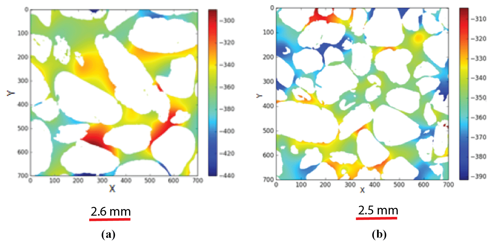
Figure 8Electrical potential field image output from the 7003 digital sub-cubes of (a) Scarborough (b) Cottesloe beaches. The colour bar indicates regions of high (red) and low (blue) potential field in arbitrary units.
The output of conductivity along the x, y, and z directions shows almost the same values of the formation factor (5.30, 4.96, and 5.08, respectively). The difference in the values of formation factor between the x direction and y direction is 6.6 %, while that between the x direction and z direction is 4.4 %; hence, the sample presents a small anisotropy at the scale of investigation. In the following, we took an average of the conductivities in the three different directions, which mathematically is equal to one-third of the trace of the conductivity tensor; for simplicity, we then consider the conductivity to be a scalar number for all images.

Figure 9Electrical potential field images (a) along the x direction, (b) along the y direction, and (c) along the z axes.
From the effective conductivity calculated for micro-XRCT images, the electrical formation factor can be estimated as
where σw is the electrical conductivity of pore fluids, taken equal to 1 in the computation. The electrical formation factor is calculated for each of the different sub-cubes obtained from the micro-CT images of the Scarborough and Cottesloe Beach samples.

Figure 10Laboratory-measured formation factor versus porosity values for both the flow and static cells for (a) Scarborough and (b) Cottesloe Beach samples.
Table 1Summary of laboratory and micro-CT scan image results from the Scarborough Beach samples.
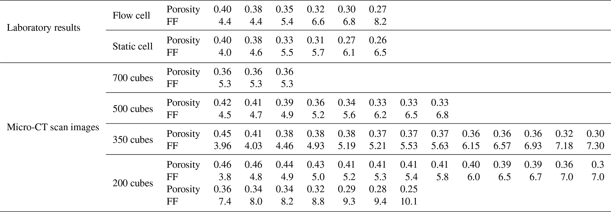
Table 2Summary of laboratory and micro-CT scan image results from the Cottesloe Beach samples.

4.1 Laboratory
Figure 10 displays the values of the formation factor against porosity for the Scarborough and Cottesloe beaches, computed as described in Sect. 2.2.2 and for each porosity value obtained by compacting the initial sand pack. Correlation coefficients were very good to excellent and varied between 0.975 and 0.999 and between 0.974 and 0.996 for the flow cell for the Scarborough and Cottesloe samples, respectively. They varied between 0.882 and 0.993 and between 0.987 and 0.999 for the static cell for the Scarborough and Cottesloe samples, respectively. The results for both the static and flow cells are reported in Tables 1 and 2 for both samples and for all data points. The values of the formation factors obtained using the flow cell are higher than those obtained using the static cell for both the Scarborough (8.2) and Cottesloe (8.5) Beach samples, whereas for Scarborough Beach, formation factors have close values at high porosities and then depart from each other at lower porosities (lower than 0.39). Some deviations between the results obtained for both static and flow cells may be due to non-uniform compaction of the samples in the case of the flow cell and/or non-complete fluid replacement in the case of the flow cell. In these figures, we have bounded the experimental data by two lines that represent a power-law relationship between the formation factor and porosity in the form
This is Archie's law (Archie, 1942) with a tortuosity factor a of 1. The tortuosity factor usually ranges from 0.5 to 1.5, but there has been quite a wide range reported in the literature for sand, from the most used value of 0.62 (Humble formula; Winsauer et al., 1952) to up to 2.45 (Porter and Carothers, 1970). We take the same tortuosity factor value of 1 for all samples. This is the value for clean granular formations (Sethi, 1979).
4.2 Micro-CT scan images
Formation factors were plotted against porosity for all the micro-CT scan image cubes for Scarborough and Cottesloe beaches (Fig. 11).
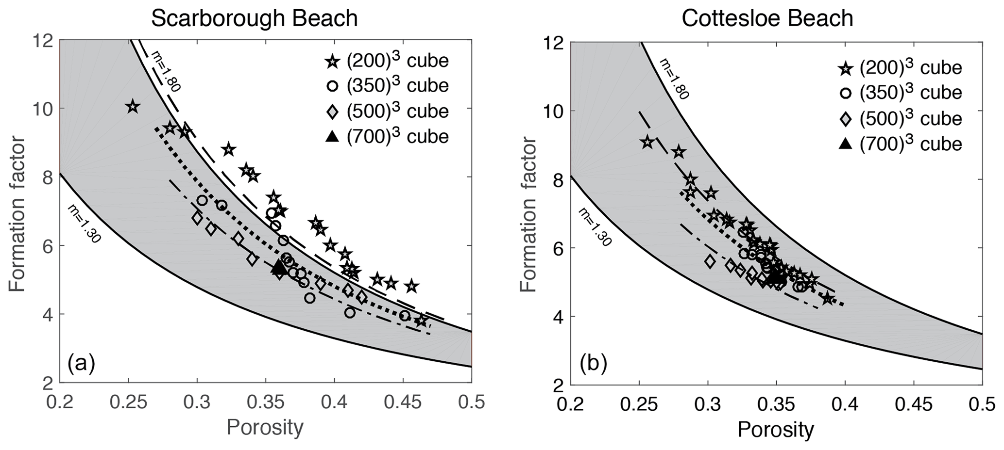
Figure 11Formation factor against porosity for each sub-cube size of 2003, 3503, 5003, and 7003 from (a) Scarborough Beach samples and (b) Cottesloe Beach samples.
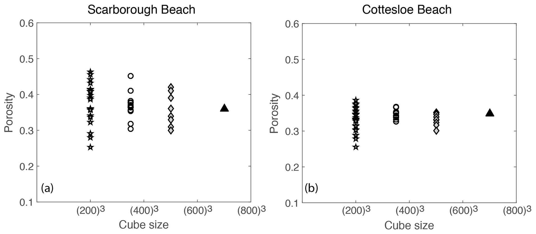
Similarly, both porosity and formation factor were plotted against the cube sizes 2003, 3503, 5003, and 7003 (Figs. 12 and 13, respectively). Scattering is shown when the cube sizes were small, which begins to level off as the representative elemental volume (REV) is approached. This REV is somewhere between 5003 and 7003, which corresponds to a sample size between 1.3 and 1.8 mm3.
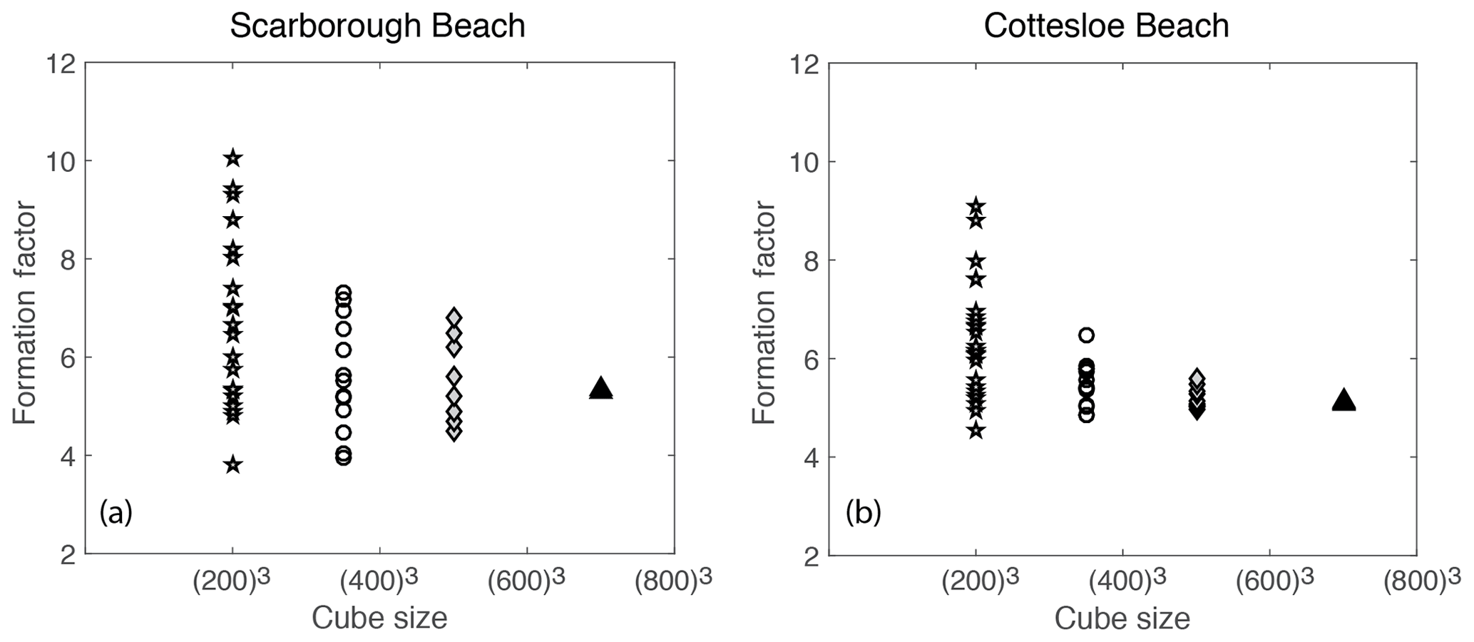
Figure 13Formation factor against cube sizes for (a) Scarborough Beach and (b) Cottesloe Beach.
As noted earlier in Sect. 4.1, the values of the formation factor obtained by the static cell are higher than those obtained by the dynamic cell (for a given porosity) for both samples. This translates into a higher cementation exponent m. One reason for this can be the design of the cell itself and the way to achieve a stable reading of sample conductivity for each fluid salinity. In the rectangular (static) cell, because the higher-salinity brine is introduced or retrieved via the centre of the panels (see Fig. 2), there could some brine left in the corners that will only equilibrate with the new injected brine by diffusion, and hence there could be a lower conductivity of the brine in these corners compared to the conductivity of the injected brine. As a result the measured sample conductivity will be lowered with respect to what it should be, giving a higher ratio of sample to brine conductivities (i.e. formation factor; see Eq. 11). Using a cylindrical cell thus has the advantage of providing a better replacement of the brine.
Figure 14 shows reported data from both the literature and those acquired in this study for the Cottesloe and Scarborough Beach samples (using the flow cell). Data from the literature include natural sand samples and synthetic granular media made of plastic particles with a regular geometrical shape (Wyllie and Gregory, 1953). We have bounded these data by the relationship presented in Eq. (14), with m=1.3, which corresponds to the original work of Archie (1942) for unconsolidated media, and by the same relationship, with m=1.8, for the upper bound. We see in this figure that our experimental results for the Cottesloe and Scarborough Beach samples are in agreement with data reported for other beach sands. Considering the data reported in this figure, we observe that Archie's classical formula for unconsolidated media underestimates the formation factor and that the departure from sphericity leads to a larger m coefficient. Since Archie's work, many authors have proposed alternative formation factor–porosity relationships. Winsauer et al. (1952) suggested that a≠1 in Eq. (14) is a better expression, whereas other authors derived a non-power-law dependency on porosity. From a practical point of view, no formula relating the formation factor to porosity for unconsolidated media fits all the experimental data, and, for a given porosity, the formation factor depends on the particle geometry, particle size distribution, and subsequent packing.
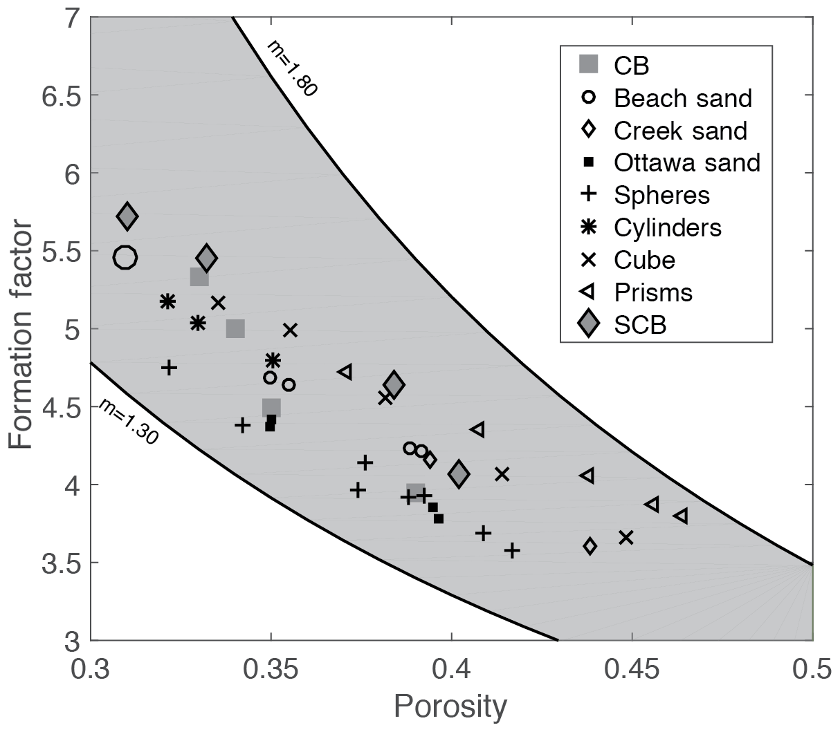
Figure 14Comparison of laboratory results with results from other researchers (Wyllie and Gregory, 1953). CB stands for Cottesloe Beach samples, and SCB is for Scarborough Beach samples.
In Fig. 15, we compare laboratory data to computed data. Laboratory data are those acquired with the flow cell, which, as discussed earlier in this section, is expected to give more reliable data. Computed data are those obtained for a cube size of 7003, which is above the REV, as presented in Sect. 4.2. We can see that there is an excellent agreement for the Cottesloe Beach sample and a good agreement for the Scarborough Beach sample. At this stage, it is difficult to explain why one sample gave better agreement and whether it is an experimental error or the higher content of carbonate grains for the Scarborough sample that makes the computation less accurate: indeed, carbonate grains may present some intra-porosity (for example, micritic phases) and thus have an electrical conductivity.
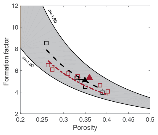
Figure 15Comparison between laboratory results (open symbols) and end-computed results (plain symbols). The trends in dashed lines are obtained from the laboratory-measured data.
The electrical properties of rocks are important parameters for well-log and reservoir interpretation. Laboratory measurements of such properties are time-consuming, difficult, and even impossible in some cases. In view of this, we have successfully combined the scientific approach of laboratory measurements (as a benchmark) with micro-CT scan computational images. We have thereby achieved the objective of determining the variability of computed formation factors as a function of porosity from laboratory measurements and micro-CT scan images from two sand samples for Scarborough and Cottesloe beaches in Perth Basin. This is the fastest method of obtaining a formation factor from CT scan images, which takes less time (5–7 h), while calculations from laboratory measurements take much more time (5 to 30 d or more).
This approach is practical, easily repeatable in real time (though expensive), and can be an alternative method for calculating a formation factor when time is not on the side of the experimenter, which is always the case. Results of images below 5003 (Scarborough) and 3503 (Cottesloe) indicate that they are not suitable REVs for pore-scale networks.
In this paper, a micro-CT scan image computational technique was employed to calculate properties such as porosity and formation factor on large three-dimensional digitized images of a sand sample. We demonstrated that for most of the parameters studied here, the values obtained by computing micro-CT scan images agreed with classical laboratory measurements and results from other researchers. This work was focused on establishing a robust methodology and workflow, and we thus started with one of the most simple materials, though it is still highly relevant for many applications in oil and gas or water management environments. For more complex geological materials, such as low-permeability rocks, multi-mineralitic rocks, and materials with conductive minerals, further developments are obviously needed. However, these developments are mostly related to the employed techniques (e.g. a higher-resolution imaging technique would be needed for low-permeability rocks, a more complex laboratory set-up, and techniques for measurements of rocks with conductive minerals or minerals with a non-negligible surface conductivity, etc.) rather than to the overall workflow established here (comparison between laboratory and computed data through trends between properties).
All data shown in Figs. 10 to 15 (except those taken from previous studies by other authors in Fig. 15 that are displayed for comparison) are given in Tables 1 and 2. X-ray images are available on request from the authors.
MAG carried out the experiments and performed the numerical simulations; SV and ML designed and planned the experiments; MM supervised and verified the numerical simulations; MAG wrote the paper in consultation with SV, MM, ML, and BG. BG initiated the project. SV conceived the original idea and supervised the project.
The authors declare that they have no conflict of interest.
We thank Dominic Howman and Vassili Mikhaltsevitch for help in cell design and laboratory experiments and Andrew Squelch for help with image processing.
This paper was edited by Ulrike Werban and reviewed by five anonymous referees.
Adler, P., Jacquin, C., and Quiblier, J.: Flow in simulated porous media, Int. J. Multiphas. Flow, 16, 691–712, 1990.
Adler, P. M., Jacquin, C. G., and Thovert, J. F.: The formation factor of reconstructed porous media, Water Resour. Res., 28, 1571–1576, 1992.
Andrä, H., Combaret, N., Dvorkin, J., Glatt, E., Han, J., Kabel, M., Keehm, Y., Krzikalla, F., Lee, M., and Madonna, C.: Digital rock physics benchmarks – Part II: Computing effective properties, Comput. Geosci., 50, 33–43, 2013a.
Andrä, H., Combaret, N., Dvorkin, J., Glatt, E., Han, J., Kabel, M., Keehm, Y., Krzikalla, F., Lee, M., and Madonna, C.: Digital rock physics benchmarks—Part I: Imaging and segmentation, Comput. Geosci., 50, 25–32, 2013b.
Archie, G. E.: The Electrical Resistivity Log as an Aid in Determining Some Reservoir Characteristics, Petroleum Transactions of the AIME, 146, 54–62, 1942.
Arns, C. H., Knackstedt, M. A., Pinczewski, W. V., and Mecke, K. R.: Euler–Poincaré characteristics of classes of disordered media, Phys. Rev. E, 63, 031112, https://doi.org/10.1103/PhysRevE.63.031112, 2001.
Auzerais, F., Dunsmuir, J., Ferreol, B., Martys, N., Olson, J., Ramakrishnan, T., Rothman, D., and Schwartz, L.: Transport in sandstone: a study based on three dimensional microtomography, Geophys. Res. Lett., 23, 705–708, 1996.
Bentz, D. P. and Martys, N. S.: Hydraulic radius and transport in reconstructed model three-dimensional porous media, Transport Porous Med., 17, 221–238, 1994.
Constable, S. and Srnka, L. J.: An introduction to marine controlled-source electromagnetic methods for hydrocarbon exploration, Geophysics, 72, WA3–WA12, 2007.
Dunsmuir, J., Ferguson, S., and D'Amico, K.: Design and operation of an imaging X-ray detector for microtomography, Photoelectric Image Devices, the McGee Symposium, Imperial College, London, 2–6 September 1991, 257–264, 1991.
Dvorkin, J., Derzhi, N., Diaz, E., and Fang, Q.: Relevance of computational rock physics, Geophysics, 76, E141–E153, 2011.
Fredrich, J., Menendez, B., and Wong, T.: Imaging the pore structure of geomaterials, Science, 268, 276–279, 1995.
Garboczi, E. J.: Finite Element and Finite Difference Programs for Computing the Linear Electric and Elastic Properties of Digital Images of Random Materials, NIST Interagency/Internal Report (NISTIR) – 6269, Maryland, United States, 1998.
Garrouch, A. A. and Sharma, M. M.: The Influence of clay content, salinity, stress, and wettability on the dielectric properties of brine-saturated rocks: 10 Hz to 10 MHz, Geophysics, 59, 909–917, 1994.
Guéguen, Y. and Palciauskas, V.: Introduction to the physics of rocks, Princeton University Press, New Jersey, 1994.
Jinguuji, M., Toprak, S., and Kunimatsu, S.: Visualization technique for liquefaction process in chamber experiments by using electrical resistivity monitoring, Soil Dyn. Earthq. Eng., 27, 191–199, 2007.
Johnson, D. L. and Sen, P. N.: Dependence of the conductivity of a porous medium on electrolyte conductivity, Phys. Rev. B, 37, 3502–3510, 1988.
Joshi, M. Y.: A class of stochastic models for porous media, University of Kansas, Lawrence, 1974.
Miller, M. N.: Bounds for effective electrical, thermal, and magnetic properties of heterogeneous materials, J. Math. Phys., 10, 1988–2004, 1969.
Miller, R. L., Bradford, W. L., and Peters, N. E.: Specific conductance: theoretical considerations and application to analytical 100 quality control, Water Supply Paper, 2311, https://doi.org/10.3133/wsp2311, 1988.
Milton, G. W.: Bounds on the elastic and transport properties of two-component composites, J. Mech. Phys. Solids, 30, 177–191, 1982.
Mitsuhata, Y., Uchida, T., Matsuo, K., Marui, A., and Kusunose, K.: Various-scale electromagnetic investigations of high-salinity zones in a coastal plain, Geophysics, 71, B167–B173, 2006.
Nakashima, Y. and Nakano, T.: Accuracy of formation factors for three-dimensional pore-scale images of geo-materials estimated by renormalization technique, J. Appl. Geophys., 75, 31–41, 2011.
Øren, P.-E. and Bakke, S.: Process based reconstruction of sandstones and prediction of transport properties, Transport Porous Med., 46, 311–343, 2002.
Øren, P. E., Bakke, S., and Held, R.: Direct pore-scale computation of material and transport properties for North Sea reservoir rocks, Water Resour. Res., 43, W12S04, https://doi.org/10.1029/2006WR005754, 2007.
Porter, C. R. and Carothers, J. E.: Formation factor-porosity relation from well log data: Soc. Professional Well Log Analysts, 11th Ann. Logging Symp., Trans., Paper D, 1970.
Schlüter, S., Sheppard, A., Brown, K., and Wildenschild, D.: Image processing of multiphase images obtained via X-ray microtomography: a review, Water Resour. Res., 50, 3615–3639, 2014.
Schwartz, L., Auzerais, F., Dunsmuir, J., Martys, N., Bentz, D., and Torquato, S.: Transport and diffusion in three-dimensional composite media, Physica A, 207, 28–36, 1994.
Sethi, S. P.: A Conceptual Framework for Environmental Analysis of Social Issues and Evaluation of Business Response Patterns, The Academy of Management Review, 4, 64–74, 1979.
Spanne, P., Thovert, J., Jacquin, C., Lindquist, W., Jones, K., and Adler, P.: Synchrotron computed microtomography of porous media: topology and transports, Phys. Rev. Lett., 73, 2001–2004, 1994.
Torquato, S.: Thermal conductivity of disordered heterogeneous media from the microstructure, Rev. Chem. Eng., 4, 151–204, 1987.
Vialle, S.: Etude expérimentale des effets de la dissolution (ou de la précipitation) de minéraux sur les propriétés de transport des roches, PhD thesis, IPG Paris and Paris-Sorbonne Denis Diderot VII, France, 2008.
Wyllie, M. R. J. and Gregory, A. R.: Formation factors of unconsolidated porous medium: influence of practical shale and effect of cementation, Transactions of the American Institute of Mechanical Engineers, 198, 103–110, 1953.
Winsauer, W. O., Shearing, H. M., Masson, P. H., and Williams, M.: Resistivity of brine saturated sands in relation to pore geometry, AAPG Bulletin, 36, 253–277, 1952.
Yeong, C. and Torquato, S.: Reconstructing random media, Phys. Rev. E, 57, 495–506, 1998.
Zhan, X. and Toksoz, M. N.: Effective Conductivity Modeling of a Fluid Saturated Porous Rock, Massachusetts Institute of Technology, Earth Resources Laboratory, Cambridge, 2007.