2.1 Inversion methodology

The inversion procedure we propose integrates spatially varying prior information to weight the regularization function locally (e.g. in each cell). It is implemented in an expanded version of the least-square inversion platform TOMOFAST-X (Martin et al., 2013, 2018), which offers the possibility to condition the regularization function (Tikhonov and Arsenin, 1977) of Li and Oldenburg (1996) locally using geological uncertainty. This is achieved by incorporating prior information into a structure-based regularization function in a fashion similar to Brown et al. (2012), Wiik et al. (2015) and Yan et al. (2017) by locally adjusting the related weight.

Solving the inverse problem regularized in this fashion consists of finding a model m that minimizes the objective function θ given below:

where d relates to the geophysical measurements to be inverted, g is the forward modelling operator, m relates to the model being searched for, and m_p is the prior model; W_d, W_m and W_H are diagonal weighting matrices corresponding to data noise, model weighting and gradient regularization, respectively. The model term is a ridge regression constraint term (Hoerl and Kennard, 1970).

The structural regularization term in Eq. (1) enforces structural constraints during inversion. It is weighted locally by matrix W_H, which can be derived from prior information (see Sect. 2.3 for details). The positive free parameters α_m and α_H control the overall weight of model and structural regularization terms; ∇ is the spatial gradient operator. Note that $|\mathrm{\nabla }m{|}_{\mathrm{2}}$ estimates the amount of structure in inverted physical property model m. Also note that parts of the model where W_H=0 are excluded from the calculation of the structural regularization and can change freely to accommodate geophysical data.

We utilize the integrated sensitivity technique of Portniaguine and Zhdanov (2002) to balance the decreasing sensitivity of gravity data with depth. We chose this technique because it offers the advantage of providing “equal sensitivity of the observed data to the cells located at different depths and at different horizontal positions” (Vatankhah and Renaut, 2017).

2.2 Probabilistic geological modelling

Probabilistic geological modelling is performed using the Monte Carlo uncertainty estimator (MCUE) method of (Pakyuz-Charrier et al., 2018a, b), which extends previous works from Jessell et al. (2010), Lindsay et al. (2012) and Wellmann et al. (2010). It is a 3-D uncertainty propagation method for implicit geological modelling that uses geological rules and geological orientation measurements (foliation and interface of the geological units sampled at surface level or in boreholes) as inputs. The sampling algorithm perturbs orientation data used to derive a reference model by sampling probability distributions describing the uncertainty of orientation data to produce a series of unique altered geological models. Realizations that do not respect a series of geological rules are considered implausible and are rejected. Coupled to the 3-D geological modelling engine of Geomodeller© (Calcagno et al., 2008), it produces a set of plausible geological models honouring the geological input measurements that represent the geological model space (Lindsay et al., 2013b). The observation probabilities constituting the probabilistic geological model (PGM) are obtained, in each model cell, by calculating the relative observation frequencies of the different lithologies from the set of geological models. For the ith model cell of a PGM containing L lithologies, vector ${\mathit{\psi }}^i=[{\mathit{\psi }}_{k=\mathrm{1}}^i$, …, ${\mathit{\psi }}_{k=L}^i]$ contains the observation probabilities of each lithology. As we show in the next subsection, the resulting PGM can be used to estimate uncertainty levels and as a source of prior information.

2.3 Utilization of information entropy for local conditioning

Information entropy was introduced for geological modelling by Wellmann and Regenauer-Lieb (2012) and is gaining popularity as a measure of uncertainty in probabilistic geological modelling (de la Varga et al., 2018; de la Varga and Wellmann, 2016; Lindsay et al., 2013, 2014; Pakyuz-Charrier et al., 2018b; Schweizer et al., 2017; Thiele et al., 2016; Wellmann et al., 2017; Yamamoto et al., 2014). Quoting Schweizer et al. (2017), information entropy “quantifies the amount of missing information and hence, the uncertainty at a discrete location”. For the ith model-cell, it is given as follows (Shannon, 1948):

Fundamentally, geological uncertainty contained in H encapsulates information about possible locations of interfaces between units and areas where the geological data are insufficiently informative. Instead of using H directly, we calculate W_H by utilizing its normalized complementary, which reflects the degree of certainty across the model. Let us express W_H as follows, for the ith model cell:

The consequence of Eqs. (2) and (3) is that W_H is minimum at interfaces and in areas poorly constrained by geological information, and equal to unity in areas where the geology is well resolved. Consequently, the conditioning process attaches small weights to the structural term of Eq. (1) in uncertain cells, while consistently high values will be applied to the most geologically certain cells. As a result, it enables the inversion algorithm to favour nearly constant changes in the inverted model in certain contiguous groups of cells (e.g. where W_H→1) while relaxing the regularization constraints in the most uncertain parts (e.g. where W_H→0).

3.1 Survey set-up

The 3-D unperturbed reference geological model was generated from contact (interface points) and surface orientation (foliations) field measurements collected in the Mansfield area (Victoria, Australia). It presents a Carboniferous mudstone–sandstone basin oriented 170^∘ north, abutting a faulted contact with a folded ultramafic basement to the south-west. Model complexity was artificially increased through the addition of a north–south fault and of a mafic intrusion.

The true density contrast model (Fig. 1a) was obtained by assigning density contrasts consistently with the structural setting of the reference geological model, assuming a flat topography. Density contrasts of 0 and 100 kg m⁻³ were assigned to the upper and lower basin lithotypes, respectively. Mafic rocks were assigned a density contrast of 200 kg m⁻³ while the density contrast of the ultramafic basement was set to 300 kg m⁻³.

Figure 1True density contrast model and W_H values used for local regularization conditioning. (a) Unperturbed reference model populated with density contrast values, (b) uncertainty values used for local regularization conditioning.

Download

MCUE perturbations of the reference geological model were first performed using standard measurement uncertainty values recommended by metrological studies, as reported by Allmendinger et al. (2017) and Novakova and Pavlis (2017). We generated a series of 300 models that were subsequently combined into a PGM. The resulting volume representing the W_H values calculated from this PGM in each cell of the model as per Eq. (3) is shown in Fig. 1b.

3.2 Locally constrained inversion: validation

To assess the impact of local conditioning of the regularization function onto inversion, we compare inversions using a non-conditioned (Fig. 2a) and a locally conditioned (Fig. 2b) regularization function, respectively. Please note that when simulating the absence of prior petrophysical information, a homogenous prior model set to 0 kg m⁻³ was used in both cases.

Besides qualitative visual comparison of the models, we interpret inversion results (Fig. 2) through the commonly used model and data root-mean-square errors (RMSEs), which correspond to the model and data terms calculated with weights and covariances set to unity. We evaluate the geometrical similarity between inverted and true model through the Bravais–Pearson correlation (also often called “linear correlation coefficient”) between their gradients (Table 1).

Table 1Indicators for comparison of inversion results in terms of model, data and structure.

Download Print Version | Download XLSX

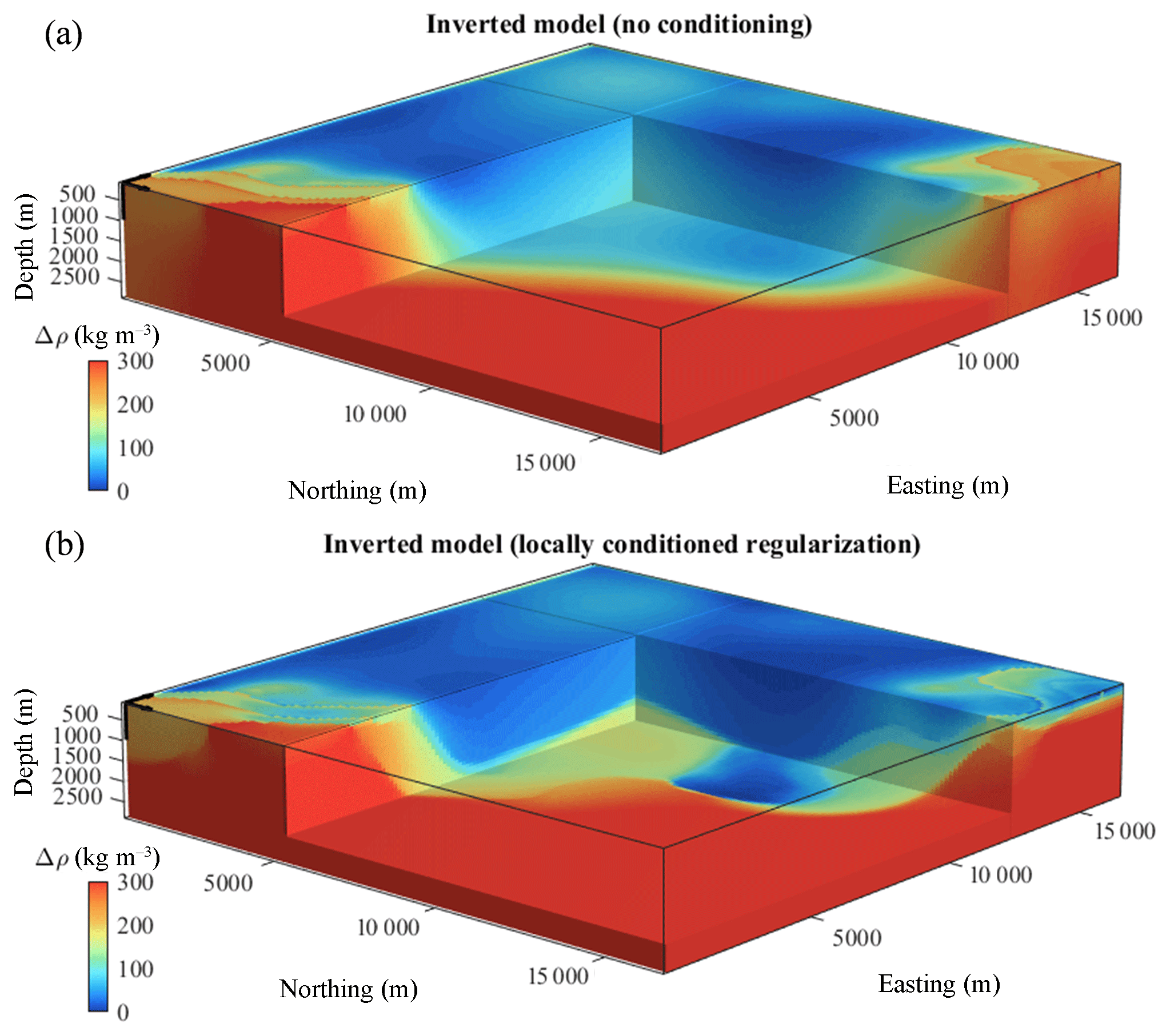
Figure 2Comparison of inversion results. (a) Inverted models with non-conditioned regularization weights, and (b) using local conditioning.

Download

Comparison of the true model (Fig. 1a) with inversion results in Fig. 2a and b shows that, while the structures in the shallowest part of the model are well retrieved in both cases, it appears that they are considerably better recovered through usage of conditioned regularization overall (Fig. 2b). The guiding effect of W_H is visible in Fig. 2b where the main structures at depth follow the general features of the conditioning volume (Fig. 1b). Moreover, in order to minimize the conditioned regularization constraint simultaneously to data misfit, inversion was driven to accommodate inverted model values (Fig. 2b) such that they are closer to the causative model (Fig. 1a) than without conditioning (Fig. 2a). This leads to reduced model RMSE on the one hand, and increased data RMSE on the other (Table 1). This reduction in data RMSE can also be explained by the relaxation of the constraints in several portions of the model, thus increasing the degree of liberty to accommodate the model towards lower data misfit. More importantly, the Bravais–Pearson correlation between the inverted and true model gradients is much higher when information from information entropy is used. This indicates that local conditioning of the regularization function also allows for significantly better retrieval of the causative bodies' (e.g. the true model) structural features.

Please also note that we do not show the recovered geophysical measurements because visual differences between recovered and inverted measurements are minimal.

From these observations, we conclude that the application of the local conditioning scheme can fulfil the objectives of data integration in inversion as it allows inversion to recover models that are closer to the causative bodies and easier to interpret, while honouring geophysical data. Nevertheless, it remains important to test the methodology in cases where the uncertainty indicator W_H is biased and/or shows high-geological-uncertainty levels away from faults and contacts. As a thorough analysis lies beyond the scope of this paper, the remainder of this section presents an elementary sensitivity analysis using a series of two W_H volumes representing distinct extreme scenarios.

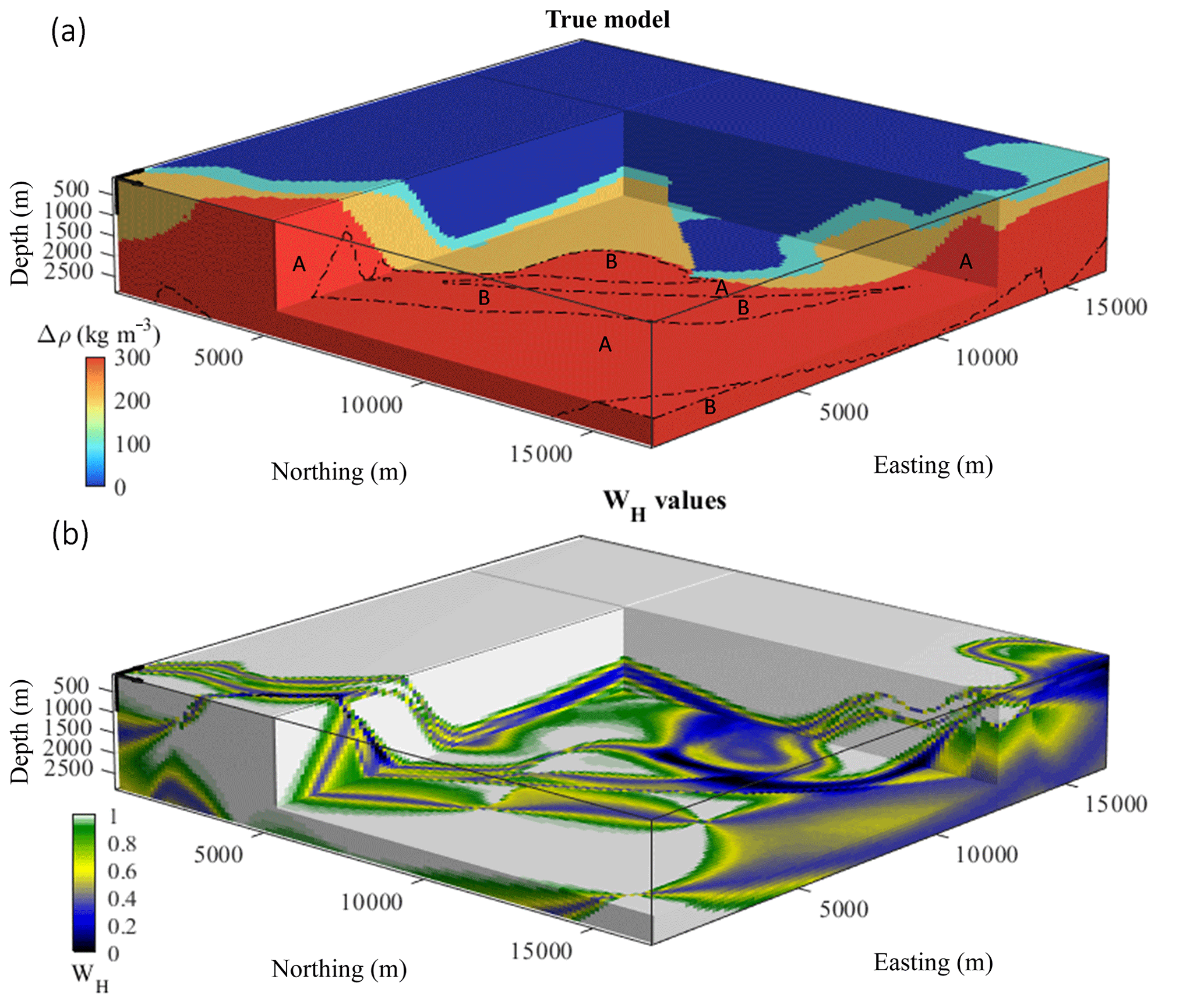
Figure 3(a) True density contrast model with outline of the “ghost” unit B (black dashed line), embedded in ultramafic unit A, and (b) local weights calculated from the PGM calculated using MCUE for model (a).

Download

3.3 Inversion constrained by biased geological uncertainty model

In this subsection, we investigate the effect of inaccurate geological models and the propagation of the related uncertainty in inversion. For this purpose, we calculate a second PGM from MCUE perturbations in which we split the ultramafic basement into two independent units, without changing the density contrast values (Fig. 3a). This results in the existence of a fictitious geological unit that is invisible to gravity data and presents no density contrast but which increases geological complexity and uncertainty (Fig. 3b) (we further refer to it as a “ghost” geological unit). Notably, it increases geological uncertainty and smears interfaces that are well-constrained as per Fig. 1. It also decreases W_H in large parts of the model where W_H→1 previously, thereby favouring model changes in these areas during inversion and encouraging it to place larger density contrast or interfaces in these areas.

Comparison of the inverted models obtained without (Fig. 4a) and with the ghost unit (Fig. 4b) reveals that they exhibit broadly similar features except in the most geologically complex parts of the model as per Fig. 1b, where differences are minor. This indicates that while geophysical inversion updates the prior density contrast model preferably in geologically uncertain regions, low values of W_H do not necessarily lead to the modelling of an interpretable interface by inversion. From the comparison of Figs. 3b and 4b, we can deduce that local conditioning as applied in this work does not necessarily enforce strict structural similarity between the inverted model and the conditioning geological uncertainty volume.

3.4 Inversion constrained using exaggerated geological uncertainty

To complete this series of tests, we generated a third PGM showing exaggerated geological uncertainty. To this end, we used a half-aperture 95 % confidence interval of ∼50^∘ for orientation data measurements in our MCUE simulations. This is far higher than for the rest of the MCUE simulations used in this paper. All other simulations (Sect. 3.2 and 3.3) use a value of ∼11^∘, which is representative of realistic measurement uncertainty as proposed by recent metrological studies (Allmendinger et al., 2017; Cawood et al., 2017; Novakova and Pavlis, 2017). Figure 5 shows the resulting W_H volume (Fig. 5a) and the inverted model obtained by using it for local conditioning of the regularization constraint (Fig. 5b).

The features visible in Fig. 5a reflect the high geological input measurement uncertainty. Geologically uncertain areas cover large portions of the volume and only the simplest geological structures (e.g. the basin) seem to be well constrained by geology. Areas of the model previously well constrained (Fig. 1b) present varying degrees of uncertainty. This illustrates that, as can be expected, increasing geological input uncertainty translates in relaxing the guiding effect of local conditioning using W_H, which results in geophysical inversion being less strongly guided by geological information. As can be seen in Fig. 4b, the inverted model obtained in this case shows structures that present weaker contrast around interfaces than when geological uncertainty is lower (Fig. 2b). Importantly, however, most structures are well preserved and the overall model values for the different lithologies remain closer to the true model than for the non-conditioned case (Fig. 2a). This indicates that even in high geological uncertainty scenarios, interpretation outcome may be largely more reliable when local regularization is used.

Figure 4Comparison of inverted model using W_H derived from a PGM considering the ghost unit (b) and without it (a); (a) is the inverse model obtained without bias in the PGM as per Fig. 2 and is shown here for comparison with (b).

Download

The analysis and comparison of the results shown in this section demonstrates the potential of the proposed inverse modelling scheme to ameliorate inversion results and to reduce interpretation uncertainty. It also illustrates the capability of our methodology to deal with high or biased conditioning uncertainty estimates. In this synthetic case, local conditioning allows geophysical inversion to significantly improve the imaging of geologically uncertain areas and to exploit complementarities between geological modelling and geophysical inversion. From the success of this proof-of-concept study, we are confident that our integration method can be tested here using real world data for field validation.

4.1 Geological context and geophysical survey set-up

The Yerrida Basin is located in the southern part of the Capricorn Orogen, at the northern margin of the Yilgarn Craton in Western Australia (Fig. 6a), and extends approximately 150 km N–S and 180 km E–W (Fig. 6b). The studied area is bounded in the north-west by the Goodin Fault, which represents a faulted contact between the Yerrida Basin and the Bryah–Padbury Basin. The structures of interest in this work are the Archean greenstone belts extending north-northwest that are unconformably overlain by Paleoproterozoic sedimentary rocks the form the Yerrida Basin. Features A and B (Fig. 6a and b) indicate the interpreted position of buried Wiluna Greenstone Belt. Where the Wiluna Greenstone Belt is exposed, it is host to base and precious metal mineralization (Williams, 2009). With a relatively high positive density contrast (expected to be between 190 and 270 kg m⁻³) to the Yilgarn Craton granite–gneiss host, mafic greenstone belts A–C are suitable targets for gravity inversion. Interpretations from multiple studies in the region, e.g. Johnson et al. (2013), Pirajno et al. (1998), Pirajno and Adamides (2000), and Pirajno and Occhipinti (2000) were compiled, while additional geological measurements acquired in 2015–2017 complemented legacy data (Occhipinti et al., 2017; Olierook et al., 2018). This allowed the revision of existing models and improved our understanding of the area. This, in turn, also highlights the challenges presented by the characterization of greenstone belts A–C, and that further geophysical analysis through constrained inversion is a useful pathway for reducing exploration risk.

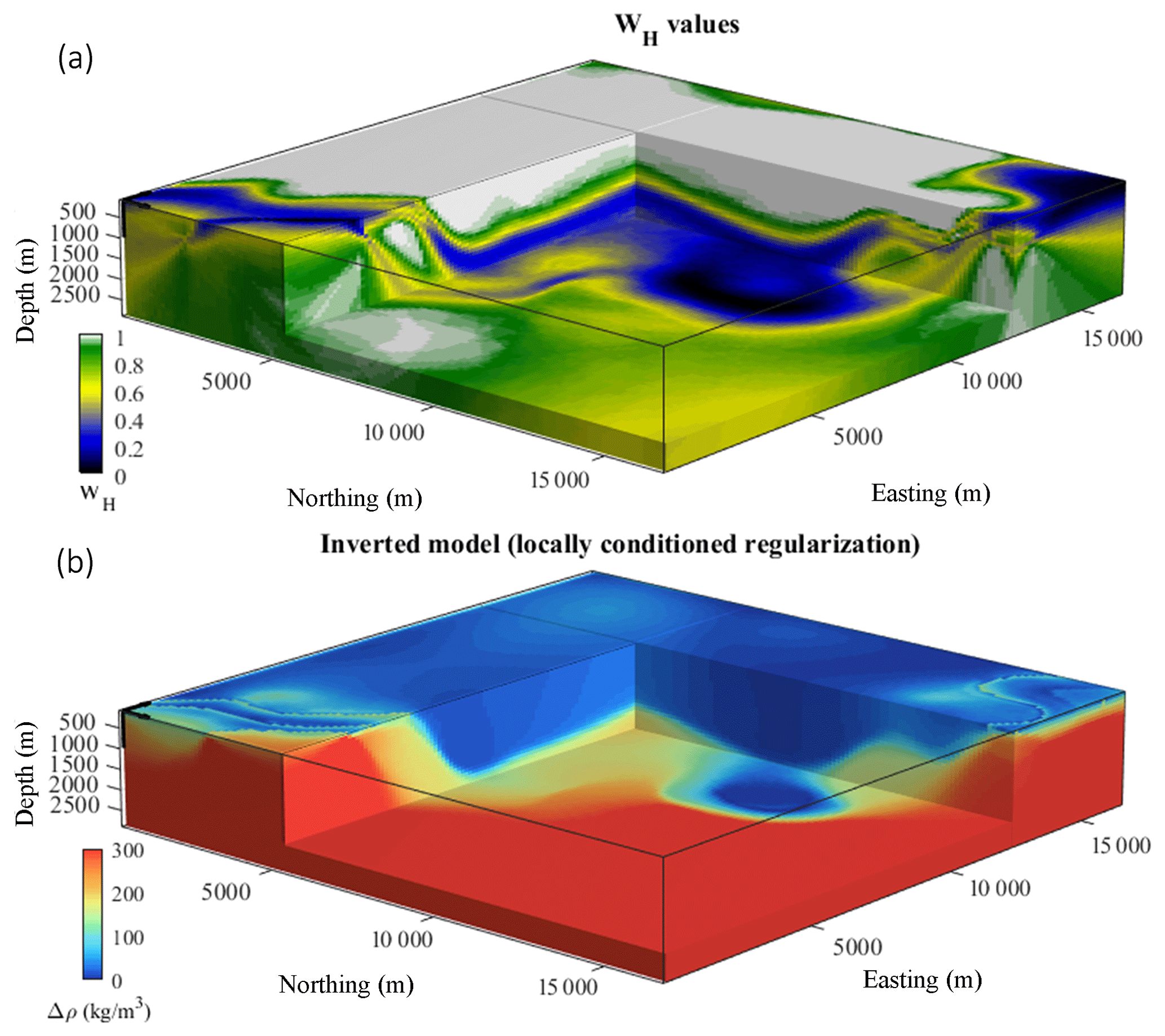
Figure 5(a) Local weights W_H calculated from a PGM, corresponding to exaggerated uncertainty in geological input measurements and (b) corresponding inverted density contrast model.

Download

Geophysical data consist of ground surveys obtained from Geoscience Australia (http://www.ga.gov.au/data-pubs, last access: November 2018). Post-processing includes spherical-cap and terrain corrections and the removal of the regional trend to obtain the complete Bouguer anomaly. As most data points were acquired 1 to 4 km apart, the dataset was resampled to match the geological model discretization, making up a total of 4882 measurement points. The model is discretized into $\mathrm{100}\times \mathrm{100}\times \mathrm{42}$ cells of dimensions 2.335 km × 1.875 km × 1.0475 km, down to a depth of 44 km, making up a total of 420 000 cells.

4.2 Geological modelling

Geological information consists of in situ structural measurements (interfaces and foliations) and interpretation of aeromagnetic, airborne electromagnetic, Landsat 8 and ASTER hyperspectral data. Legacy data from the Geological Survey of Western Australia (Pirajno and Adamides, 2000) and CSIRO (Ley-Cooper et al., 2017) were used, to which about 600 surface geological and petrophysical measurements from recent geological field campaigns were added. Although the available petrophysical measurements were not used to derive petrophysical constraints because of the insufficient sampling of several of the modelled lithologies, they were a useful source of information to populate geological models and for interpretation. Remote-sensing data were used to test interpretations.

These datasets were used jointly to build a reference geological model reconciling the available geological information in Geomodeller.

Lithologies with similar density contrasts were merged and subsequently treated as a single rock type in MCUE simulations. Uncertainty related to structural measurements was subsequently used as inputs to the MCUE perturbations (Pakyuz-Charrier et al., 2018b) of the reference model to generate a collection of 500 accepted models. Information extracted from the PGM is displayed in Fig. 7. Figure 7a shows the lithologies with the highest probability for each cell of the PGM. The associated W_H values used in inversion are shown in Fig. 7b. The prior model for inversion m_p is equal to the mean model of the 500 plausible models generated by MCUE. It is shown in Fig. 7c.

4.3 Inversion results and analysis

The aim of our analysis is to assess the influence of the local conditioning of structural constraints on inversion through comparison with the non-conditioned case, all other things remaining constant.

Figure 6Geological context and geophysical data. (a) Geological map of the area and (b) complete Bouguer anomaly. The dashed lines delineate the possible sub-basin extent of the mafic greenstone belts A–C.

Download

4.3.1 Comparative analysis strategy

Prior to examination of the inverted models, we analyse geophysical data misfit after inversion. This enables us to ensure that the inversion results we compare produce, in our case, similar gravity anomalies. Our study of inverted models focuses on results obtained through usage of non-conditioned (Fig. 8a) and conditioned regularization functions (Fig. 8b) using W_H (Fig. 7b). In addition to departures from the prior model, variations between the two cases are studied by visual comparison of Figs. 8a and 7b, through qualitative (Fig. 7c) and quantitative comparative analysis (Fig. 7d and e). Our interpretation of inversion results is complemented by metrics quantifying the differences between models. We give particular attention to model cells where the probability of mafic greenstone is larger than zero. For these cells, we classify lithologies by identifying cells with a density contrast corresponding to mafic greenstone.

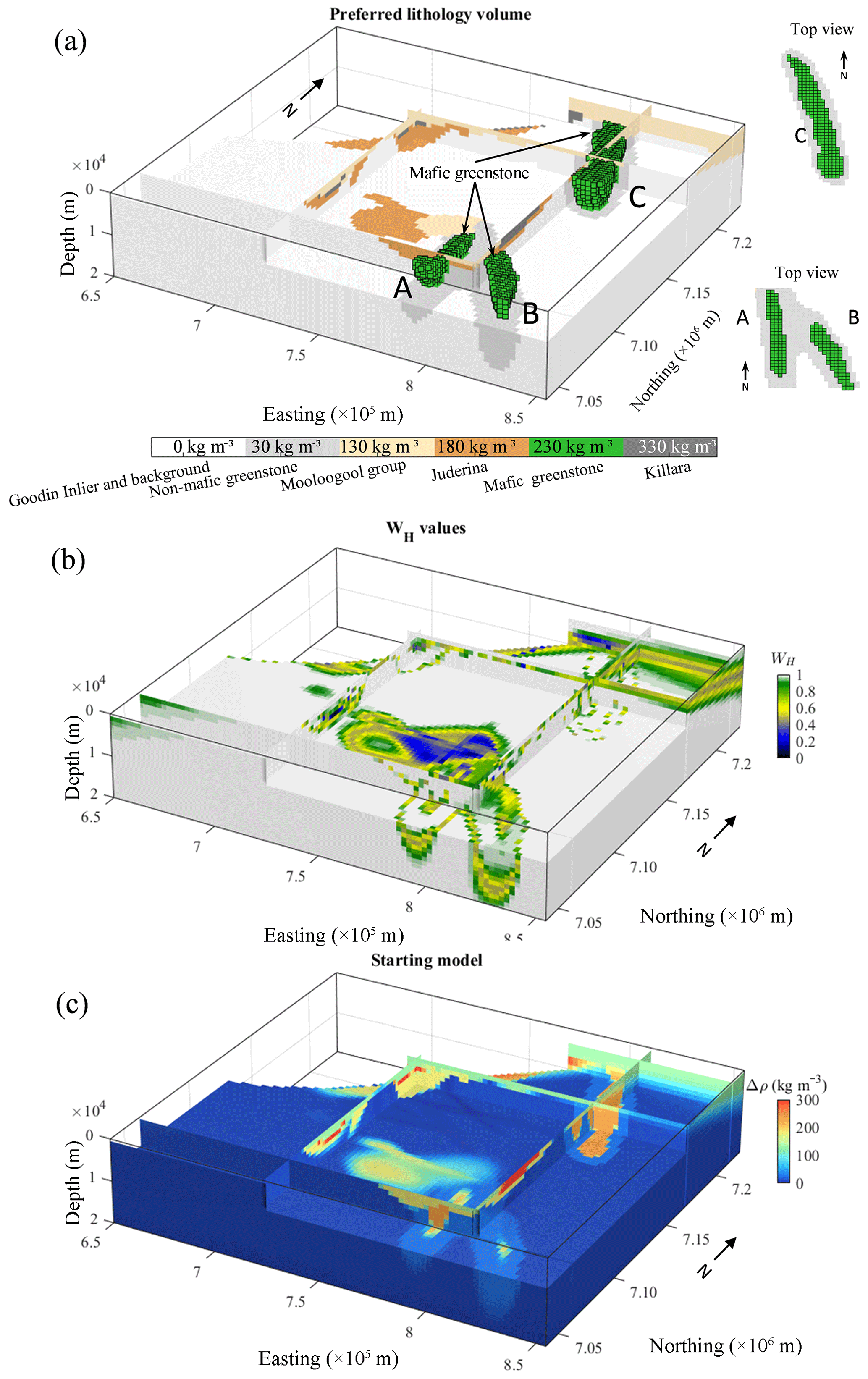
Figure 7Geological modelling results. (a) Most probable (i.e. preferred) lithology in each model cell (same colour code as in Fig. 6), (b) values used for local regularization conditioning, and (c) prior model derived from PGM and prior petrophysical information. In (a), “background” refers to all the lithologies that have a density contrast equal to 0 kg m⁻³.

Download

4.3.2 Results

Data root-mean-square (RMS) error decreases during inversion from 12.46 mGal to reach 1.59 and 1.53 mGal for the non-conditioned and conditioned cases, respectively. The corresponding data misfit maps show a linear correlation coefficient of 0.999 (see details in Appendix A). This similarity illustrates that, as in many other studies, most changes related to holistic data integration in geophysical inversion occur primarily in model space, hence reducing the effect of non-uniqueness (Abtahi et al., 2016; Abubakar et al., 2012; Brown et al., 2012; Demirel and Candansayar, 2017; Gallardo et al., 2012; Gallardo and Meju, 2004, 2007, 2011; Gao et al., 2012; Giraud et al., 2017; Guo et al., 2017; Heincke et al., 2017; Jardani et al., 2013; Juhojuntti and Kamm, 2015; Kalscheuer et al., 2015; Molodtsov et al., 2013; Moorkamp et al., 2013; Rittgers et al., 2016; Sun and Li, 2016, 2017).

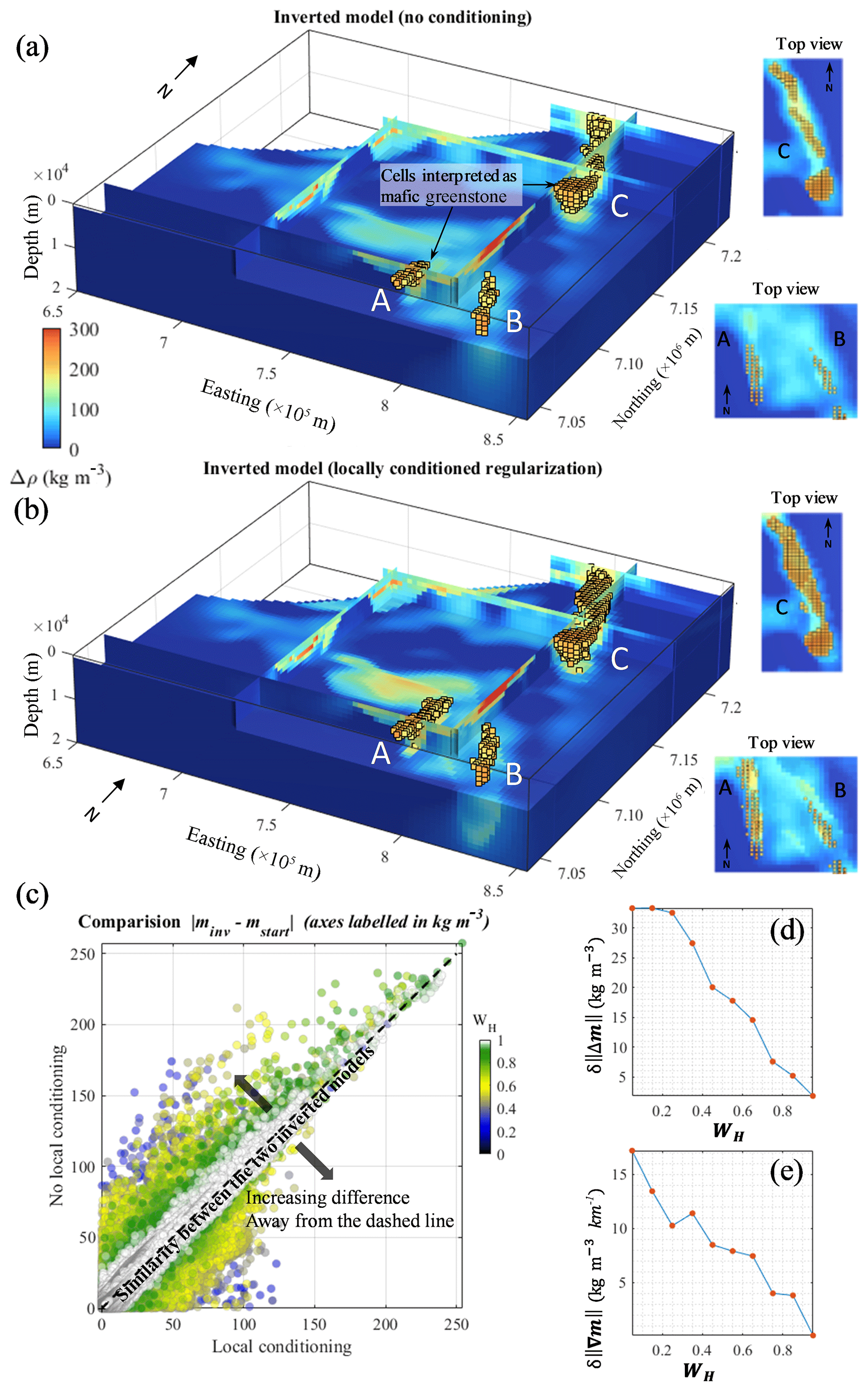
Figure 8Comparison of inversion results. (a) Inverted models with non-conditioned regularization weights, and (b) using local conditioning, (c) cross-plot between the corresponding absolute value of the update of the prior model, (d) difference in model updates $\mathit{\delta }\left|\mathrm{\Delta }m\right|=|m_{\mathrm{cond}}-m_{\mathrm{nocond}}{|}_{\mathrm{2}}$ as a function of values of W_H and (e) difference in model roughness $\mathit{\delta }\left|\mathrm{\nabla }m\right|=|\mathrm{\nabla }{m}_{\mathrm{cond}}{|}_{\mathrm{2}}-|\mathrm{\nabla }{m}_{\mathrm{nocond}}{|}_{\mathrm{2}}$ as a function of values of W_H. The model cells labelled A–C are interpreted as mafic greenstone belts. All voxels are coloured as a function of density contrast.

Download

Qualitatively, comparison of Fig. 8a and b reveals that departures from the prior model (Fig. 7c) are more significant in the most geologically uncertain areas. Quantitatively, the RMS model update for cells characterized by $\mathrm{0}\le W_{\mathrm{H}}<\mathrm{0.05}$ (most uncertain group) is equal to 40.1 and 51.5 kg m⁻³, for the non-conditioned and conditioned cases, respectively, whereas the same quantities are equal to 17.7 and 16.9 kg m⁻³ for the cells identified by $\mathrm{0.95}<W_{\mathrm{H}}\le \mathrm{1}$ (most certain group). This suggests that local regularization conditioning allows inversion to update the model preferentially in geologically uncertain areas. In turn, differences with the prior model in more geologically certain areas are reduced compared to the non-conditioned case. This effect of conditioning is corroborated by Fig. 8c, in which the longest distances to the dashed line, which represents equal model update for the two studied cases, occur in geologically uncertain areas. This also translates into a higher difference between model updates of the two cases in Fig. 7d for lower values of W_H. In addition, we observe that local conditioning produces stronger density contrasts in Fig. 8b in some of the areas where the conditioning values are higher in Fig. 8b. Furthermore, structures in the inverted model are easier to identify when local conditioning is used. It is confirmed by global roughness measures $|\mathrm{\nabla }m{|}_{\mathrm{2}}$ equal to 3.4 and 4 ( (kg m⁻³ m⁻¹) for the non-conditioned and conditioned cases, respectively. More specifically, as shown by Fig. 7e, this difference arises in parts of the model associated with lower W_H, which characterize uncertain areas, including interfaces between lithologies.

The recovered greenstone belts are shown in Fig. 8a and b. In Fig. 8b, the extension of recovered mafic greenstone belts is significantly different than when geological uncertainty is not accounted for (Fig. 8a). In particular, belt A is significantly larger in Fig. 8b than in Fig. 8a (2.4×10² km³ vs. 4.6×10² km³). Similarly, the extent of belt C is increased overall (volume of 5.3×10² km³ vs. 14×10² km³), while its different portions reconnect; the northern half is also significantly shallower and broader than in Figs. 7a and 8a. It appears that belt A remains thinner and shallower (Fig. 8b) than suggested by the preferred lithology volume (Fig. 7a). While similar geometries for belt B are recovered in Fig. 8a and b, they both differ from Fig. 7a as only the eastern part is preserved. Note that it is larger in Fig. 8b, with a volume 40 % higher than in Fig. 8a. As discussed in the next subsection, these differences have a signification impact on the interpretation of inversion results and are important to understand the influence of local conditioning on inversion.

4.4 Interpretation

Note that, in contrast to the differences between inversion results highlighted above for belts A and C, there are only small differences between the inverted models in the north-eastern part of the model and the different interpretations of belt B (Fig. 7a and b). This shows that locally conditioned regularization does not enforce changes in the inverted model in all places where geological uncertainty is high, as uncertainty is only a reflection of potential errors. Rather, this indicates that in such cases, the guiding effect of such regularization will be exerted on the condition that it does not prevent the data term in θ(d, m) as per Eq. (1) from decreasing. This also confirms that geophysical data are the main driver of the model updates in geologically uncertain areas. Instead of smooth departures from the prior model to match geophysical data regardless of geological considerations, local regularization constraints allow inversion to account for the probabilistic geological modelling of the area and for geological uncertainty. It can therefore provide results that conform better to known geology.

In consequence, by confronting a probabilistic geological model encapsulating all MCUE realizations with geophysical measurements in an inversion scheme favouring model updates in the most geologically uncertain areas, inversion complements probabilistic geological modelling in that it guides and refines the interpretation of other geoscientific data in the area.

Geophysical inversion using geological uncertainty information (Fig. 7b) confirms the presence of high-density anomalies that we interpret to be the mafic components of the greenstone as suggested by MCUE in several portions of the model. It also adjusts the outline and geometry of belts A–C to obtain a model honouring geological uncertainty information. In particular, mafic greenstone belts A and B may be smaller than the extent suggested by the PGM, and mafic greenstone C shallower than anticipated. The interpretation of inversion results also reveals that greenstone B might extend further to the east than indicated by the preferred lithology volume (Fig. 7a) and that greenstone C may be thinner in its central part.