2.1 Governing equations

The mathematical formulation of differential movement between solid matrix and melt basically builds on that described in Schmeling (2000) and Schmeling et al. (2019) and is applied here to a porosity wave. We solve the equations for mass and momentum conservation for melt and solid. The formulation of the governing equations for the melt-in-solid two-phase flow dynamics is based on McKenzie (1984), Spiegelman and McKenzie (1987) and Schmeling (2000), and it is valid for infinite Prandtl number (i.e., neglecting inertia terms in the momentum equations), and small fluid-to-matrix-viscosity ratios. In the following all variables associated with the fluid (melt) have the subscript f and those associated with the solid have the subscript s. Without melting and freezing, the equation for the conservation of the mass of the melt is

and the mass conservation of the solid is

v_f and v_s are the fluid and solid velocities, respectively. The velocities are derived from the momentum equations, which is a generalized Darcy equation for the fluid separation flow,

and the Stokes equation for the solid–fluid mixture in the limit of zero fluid viscosity is

k_φ is the permeability that depends on the rock porosity (i.e., melt fraction) with the power n,

where η_f is the dynamic melt viscosity; g is the gravitational acceleration; ρ is the density of the melt–solid mixture, ρ_f is the density of the melt; P is the fluid pressure, whose gradient is driving the motion; and τ_ij is the effective viscous stress tensor of the matrix.

with the effective shear viscosity η_s and the effective volumetric or bulk viscosity η_b of the porous matrix. The term $\left({\mathit{\eta }}_{\mathrm{b}}-\frac{\mathrm{2}}{\mathrm{3}}{\mathit{\eta }}_{\mathrm{s}}\right)\mathbf{\nabla }\cdot {\mathit{v}}_{\mathrm{s}}$ is often referred to as compaction pressure. The linearized equation of state for the mixture density is given as

with the density of the matrix ρ_s.

The fluid pressure in Eqs. (5) and (6) is the same and can be eliminated by merging the two equations. Inserting the density of the mixture, and using Eq. (7), Eq. (5) is recast into

This equation states that the velocity difference between fluid and solid phases (i.e., fluid separation flow or the segregation velocity) is driven by the buoyancy of the fluid with respect to the solid and the viscous stress in the matrix which includes the compaction pressure.

Following Šrámek et al. (2007) the matrix velocity, v_s, can be written as the sum of the incompressible flow velocity, v₁, and the irrotational (compaction) flow velocity, v₂, as follows:

with the incompressible velocity potential or stream function ψ and the irrotational (compaction related) velocity potential, χ. From Eq. (11) it follows that the latter is given as the solution of the Poisson equation

The divergence term ∇⋅v_s can be derived from summing up Eqs. (3) and (4) to give

Equation (12) represents a Poisson equation which can be solved for χ once the melt porosity and segregation velocity are known. As boundary condition the normal velocity of v₂, i.e., v_2n, can be prescribed, which is equivalent to a normal derivative of χ, i.e., a Neuman boundary condition. If the normal velocity is constant along the boundary, it automatically fulfills free slip. For the sake of simplicity, v_2n=0  was chosen.

Taking the curl of the matrix momentum (Eq. 6) eliminates the pressure. Inserting the viscous stress tensor (Eq. 8), the density (Eq. 9) and the matrix velocity (Eq. 11) into the resulting equation gives the momentum equation in terms of the stream function ψ and the irrotational velocity potential χ

with

The governing equations are non-dimensionalized by the compaction length, δ_c0 (McKenzie, 1984), and a scaling separation velocity, v_sc0, both of which are taken at a reference state which assumes a constant background porosity φ₀. The corresponding scaling viscosities and the scaling permeability are denoted by η_b0, η_s0 and k_φ0. The compaction length is given by

and is the length scale over which a variation in fluid flux gives a response to the compaction. The scaling separation velocity is given as

This defines the scaling law, where the primes denote non-dimensional values and the subscript 0 refers to the background porosity:

The resulting governing equations for the mass are

and for the momentum equations we get

with e_z as unit vector in the z direction (positive upward).

2.2 The effective viscosity of a porous matrix

The effective viscosity laws proposed by Schmeling et al. (2012) assume ellipsoidal melt inclusions, or melt films if the inclusions are flat, or melt tubules embedded within an effective viscous medium. This self-consistent assumption is able to predict viscous weakening of a solid matrix with a disaggregation melt porosity on the order of 50 % or less depending on the assumed melt geometry. From their numerical models, Schmeling et al. (2012) derive approximate formulas for the porosity dependence of the dimensional effective matrix shear and bulk viscosities for a melt network geometry consisting of 100 % films,

with $k_{\mathrm{1}}=a_{\mathrm{1}}\left(a_{\mathrm{2}}+\mathit{\alpha }\left(\mathrm{1}-a_{\mathrm{2}}\right)\right)$, $c_{\mathrm{1}}=\frac{b_{\mathrm{1}}\mathit{\alpha }}{\mathrm{1}+b_{\mathrm{2}}{\mathit{\alpha }}^{k_{\mathrm{3}}}}$ and $c_{\mathrm{2}}=\frac{\mathrm{4}}{\mathrm{3}}\mathit{\alpha }{c}_{\mathrm{1}}^{-k_{\mathrm{2}}}\cdot \left(c_{\mathrm{3}}\left(\mathrm{1}-\mathit{\alpha }\right)+\mathit{\alpha }\right)$, where a₁=0.97, a₂=0.8, b₁=2.2455, b₂=3.45, k₂=1.25, k₃=1.29, c₃=2 and α is the aspect ratio of the ellipsoidal inclusions. At the disaggregation threshold found as φ=c₁, the partially molten material loses its cohesiveness and both viscosities approach zero.

For a melt network consisting of 50 % tubes and 50 % films, the following approximate equations have been derived from the model of Schmeling et al. (2012):

The parameters needed to calculate these viscosities for different aspect ratios between 0.2 and 0.5 are given in Table 1. k is given by $k=a_{\mathrm{1}}\mathit{\phi }+b_{\mathrm{1}}$.

Table 1Parameters to calculate the viscosities for a melt network consisting of 50 % tubes and 50 % films using Eqs. (24) and (25).

Download Print Version | Download XLSX

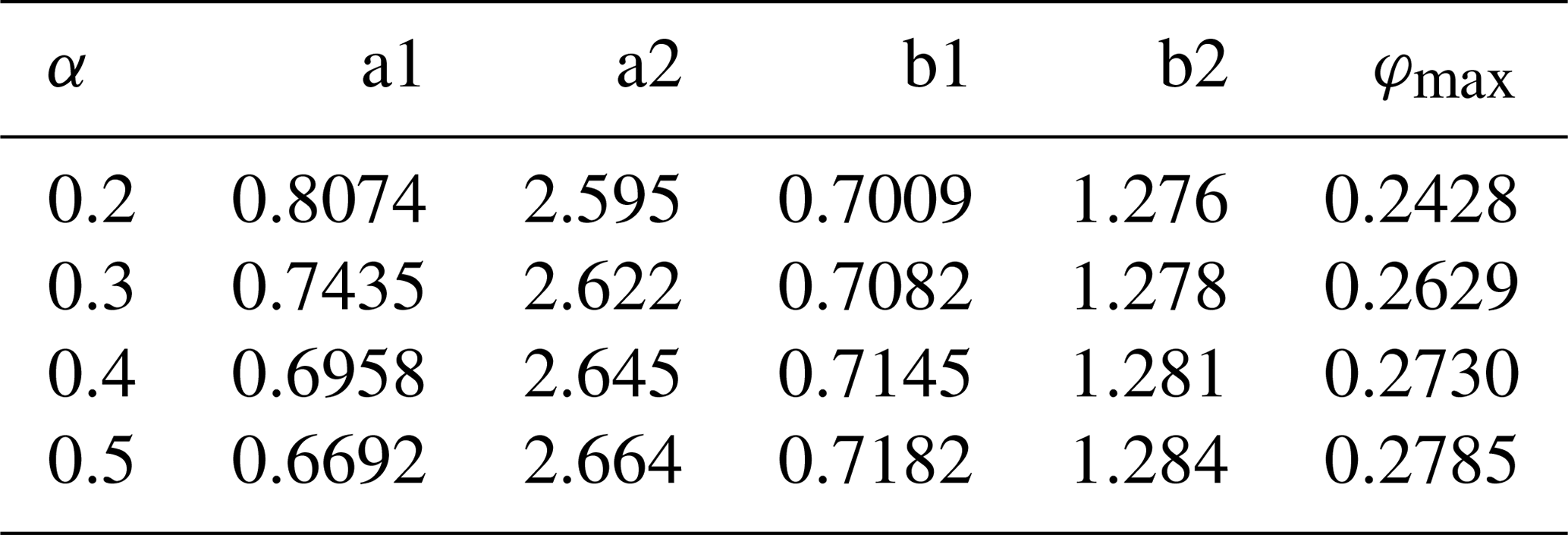
Figure 1 shows the effective shear and bulk viscosities for different aspect ratios together with the simplified previous laws (1) and (2).

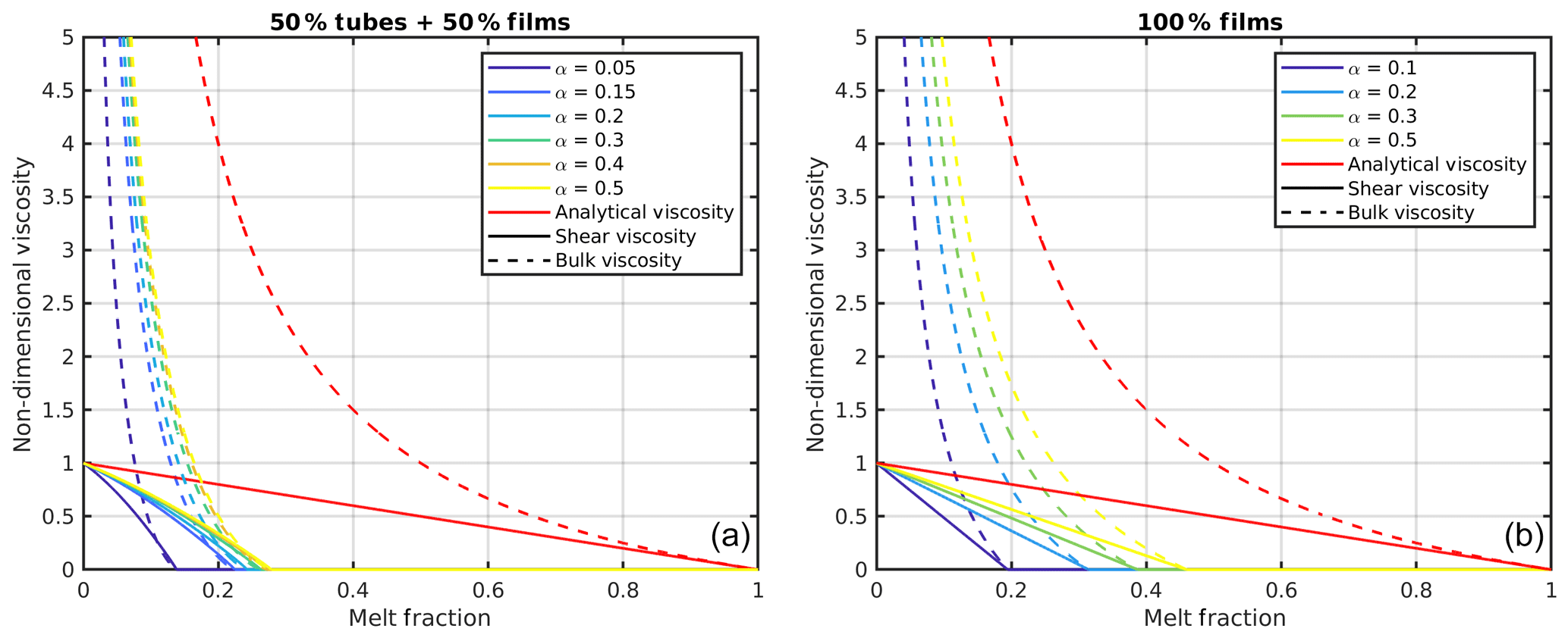
Figure 1Shear (solid) and bulk (dashed) viscosity for several aspect ratios as a function of the melt fraction. (a) The viscosities are calculated for a melt network consisting of 50 % tubes and 50 % films. (b) The network consists of 100 % films. The red lines show the simplified analytical viscosities (Eqs. 1 and 2).

Download

Takei and Holtzman (2009) and Rudge (2018) suggest that in the presence of an infinitesimal amount of connected melt the effective viscosity undergoes a finite drop on the order of a few tens of percents of the intrinsic matrix viscosity. In our approach we always have a finite melt porosity, and thus we may identify the zero porosity viscosity η_s0 in our formulation with the initially weakened value of Takei and Holtzman (2009) or Rudge (2018).

2.3 Methods and model setup

For the model we use a square box (1×1), which is initially partially molten to a certain degree, the background porosity. We place an initial porosity anomaly with a higher porosity centered at x₀=0.5 and z₀=0.2 from which a porosity wave will develop. As the shape and width of a solitary wave with a certain rheology law and amplitude is not known a priori, we use a Gaussian wave of the form

for the perturbation and vary the initial width w of the wave.

At the sides of the symmetric box boundaries and at the top and the bottom, free slip boundaries are used. The in- and outflow velocities of matrix and melt at the top and bottom are prescribed in terms of the analytical solution for the background porosity.

The influence of the boundaries on the ascending wave was investigated and found to be fairly small. In Fig. 3 one can see the effect of the upper boundary on the phase velocity. At the end, as the waves approach the upper boundary, the dispersion curves slightly deviate from the supposed line. This error is smaller than 0.5 % as long as the distance from the center of the wave to the upper boundary is greater than 1.5 times its 10 % radius. This radius is defined as the radius at which the porosity has decreased to 10 % of the amplitude of the wave. For the side boundaries this distance has to be larger. For distances greater than 3 times the 10 % radius, this error is smaller than 1 %. In our models the waves have distances of 7–10 times the 10 % radius, which correspond to errors between 0.2 % and 0.05 %.

The equations are solved on a 201×201 grid by finite differences (FDs) using the code FDCON (e.g., Schmeling et al., 2019). Resolution tests have been made with grids varying from 101×101 to 401×401. They show that after a short transient time the phase velocity and amplitude of the evolved porosity wave approach constant values for very high resolutions for all viscosity laws used. The subsequently observed slow variations in the phase velocity and amplitude of the wave along a quasi-steady-state dispersion curve can be attributed to numerical diffusion at finite grid resolution. The resolution test shows that (1) the quasi-steady-state phase velocity and amplitude of the wave are of error order 1, and (2) the dispersion curves obtained on a 201×201 grid overestimate the extrapolated phase velocity values by about 10 %. Time step resolution tests show that the long-term temporal behavior of the porosity waves is significantly improved if the time steps are chosen smaller than approximately 0.2 times the Courant criterion.

The amplitude and phase velocity of the evolving porosity wave are obtained at every time step by quadratic interpolation of the porosity values on the FD grid and determining the value and velocity of the position of the maximum of the quadratic function. The resulting phase velocity shows small oscillations in time, which are probably due to the interaction of the 1st-order error in time when solving Eqs. (3) and (4) and the 2nd-order error of the interpolation. These oscillations are smoothed by applying a moving average including 50 neighboring points. The resulting time series of porosity amplitude and phase velocity can be plotted as a curve with time as curve parameter in an amplitude–phase velocity plot. This curve can be understood as a dispersion curve because the phase velocity depends on amplitude and thus implicitly on the width or wavelength of the porosity wave.

For the model series presented below the width and the amplitude of the initial wave, the background porosity, and the rheology law have been varied. All models were carried out using n=2 and n=3 in the permeability–porosity law.

3.1 Dispersion curves for varied widths and amplitudes

As the shape of a two-dimensional porosity wave for a certain wave amplitude is not known, the initial width is varied. In Fig. 2a we show a porosity wave of amplitude 8 initially positioned at x=0.5 and z=0.2 (left) as it rises through the model box. In Fig. 2b a horizontal cross section through the maximum of an initial wave and the resulting solitary wave at a late stage are shown. During the early stage the wave gains some amplitude as the volume of an equivalent solitary wave with the same amplitude would be smaller for this example. Then the amplitude of the ascending wave slowly decreases again due to numerical diffusion and the evolving phase-velocity–amplitude curve describes the quasi-steady-state dispersion relation. At this point the wave is expected to be a solitary wave. The shape of this wave resembles a Gaussian bell-shaped curve quite well but does not fit exactly. The upper part of the wave in this example fits very well, while the lower part is slightly wider.

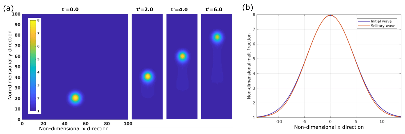
Figure 2(a) Non-dimensional melt fraction at four different time steps during the ascent of a solitary wave with an initial amplitude of 8. The model was carried out for a melt network geometry consisting of 100 % films and an aspect ratio of 0.1. The background porosity is 0.005 and n=3. (b) Horizontal cross section through the center of the initial wave and the solitary wave at a later time.

Download

To analyze the evolution of the ascending solitary wave the phase velocity and the amplitude are tracked over the full rising time and plotted into a dispersion diagram. In Fig. 3 the dispersion curves of a model with a starting wave width which is initially larger than the resulting solitary wave, a model with a similar width and a model with a smaller initial width are shown. The curves start with high velocities for the Gaussian bell-shaped wave and then rapidly slow down until they approach a specific point visible as a sharp kink from which they slowly follow a line. For the bigger and optimal width models, after this kink, the wave is expected to have reached the solitary wave stage. For the bigger initial width this stage is reached at a higher amplitude than initially assumed. It is important to note that, independent of the initial wave width, after reaching a solitary wave stage the velocities and shapes of waves of a certain amplitude are always equal, i.e., the three curves merge on one dispersion curve. For comparison with semi-analytic 2-D solitary porosity wave solutions, the dashed curves in Fig. 3 and later figures show dispersion curves with different power law n of the permeability–porosity relation and different bulk viscosity laws, with m=0 assuming a constant bulk viscosity and m=1 for a 1∕φ proportionality (see Eq. 2) (Simpson and Spiegelman, 2011). In contrast to our models, these solutions (a) use a stiff rheology (“Analytic viscosity” in Fig. 1); (b) neglect solid shear (first term of the right-hand side of Eq. 8), which is responsible for v₁ (see Eq. 12) in the matrix momentum equation and for an important contribution in the separation flow (Eq. 11); and (c) apply the small porosity limit.

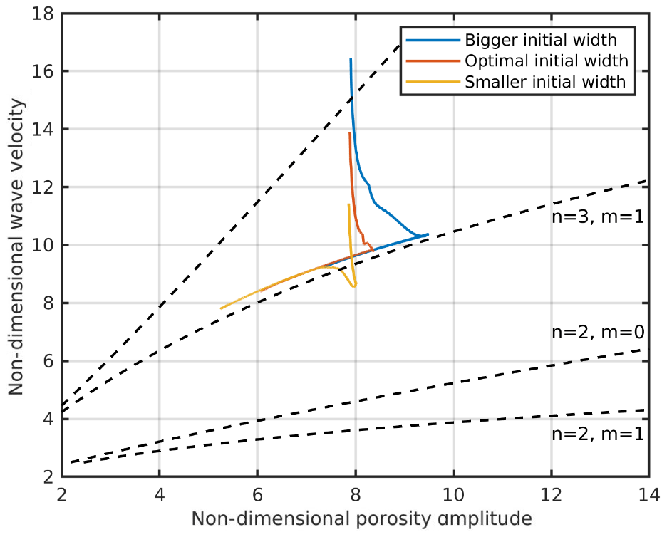
Figure 3Dispersion curves for three models with an initial width bigger, smaller and approximately equal to the resulting solitary wave. Each model was carried out for a melt network geometry consisting of 100 % films and an aspect ratio of 0.1. The background porosity is 0.005 and n=3.

Download

Based on this result one can carry out many models with different initial wave widths and different initial amplitudes and get one empirical steady-state solitary wave dispersion curve for one viscosity law for a wide range of amplitudes.

Figure 4 shows the time-dependent dispersion curves of models with four different initial amplitudes (4 to 10) and 11 different initial widths each. Depending on the initial widths, they either gain amplitudes as they approach the solitary wave stage or they monotonously loose amplitude. Depending on the initial amplitude and width, each case is characterized by a certain total melt volume, corresponding to a specific steady-state solitary wave with a specific amplitude. Therefore the 44 models finally reach one steady-state solitary wave dispersion curve at different amplitudes. As discussed in Sect. 2, the amplitudes of the waves slowly continue to decrease due to some small amount of numerical diffusion. Yet, they continue following the steady-state solitary wave dispersion curve.

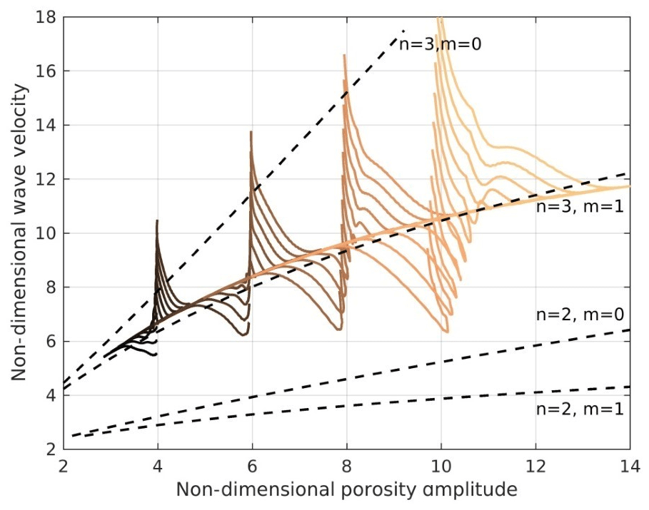
Figure 4Dispersion curves for 44 models with four different initial amplitudes (4 to 10) and 11 different initial widths each. All models were carried out for a melt network geometry consisting of 100 % films with an aspect ratio of 0.1.

Download

Although we use a different rheology law and do not apply the simplifications mentioned above, the steady-state dispersion curve of our model is in general agreement with the n=3 and m=1 dispersion curve determined semi-analytically by Simpson and Spiegelman (2011) (Fig. 4, dashed curve). However, given the 10 % numerical overestimation of phase velocities of our models (see Sect. 2.2), for high amplitudes our dispersion curve shows a significantly smaller slope and correspondingly smaller phase velocities than the semi-analytical curve by Simpson and Spiegelman (2011). Comparison of the simplified semi-analytical 1-D solution by Simpson and Spiegelman (2011) with the full analytical 1-D solution by Yarushina et al. (2015) shows that for low porosities these solutions fit very well together. For higher porosities the full solution becomes slower than the simplified one. Tentatively transferring this result to 2-D, our decrease in the slope can probably be explained by the low-porosity limitation of the Simpson and Spiegelman (2011) solution, which overestimates the velocity at high porosities.

3.2 Effect of different viscosity laws for n=2 and n=3 on dispersion curves

To investigate the effect of different viscosity laws, two melt network geometries are chosen. The first one consists of 50 % films, or ellipsoidal melt pockets, and 50 % tubes; the second of 100 % films or ellipsoidal melt pockets. Furthermore, the aspect ratio α is varied, whereby a higher aspect ratio corresponds to compact melt pockets and leads to stronger viscosities and to a higher disaggregation threshold (see Fig. 1).

Waves with these different viscosity laws give only minor differences in the dispersion curves (Fig. 5a, b). Especially with the films and tubes case, the curves for different aspect ratios (Fig. 5a) are not distinguishable, both during the transient and final stages. In contrast, the analytic viscosity case (Eqs. 1 and 2) propagates along a different path and converges to a 4 %–6 % higher final phase velocity curve. With 100 % films the differences among curves with the different viscosity laws in the final velocity are higher and lie on the order of 6 %. These differences are surprisingly small if compared to the actual differences in effective shear viscosities of about 13 % and bulk viscosity of about a factor of 4 (at 4 % melt corresponding to a porosity amplitude of 8). It is also to be noted that the steady-state part of our dispersion curve calculated with the analytical viscosity (Eqs. 1 and 2) excellently agrees with the semi-analytical solution (dashed) by Simpson and Spiegelman (2011) for the same viscosity law, if we account for the 10 % numerical overestimation of our model phase velocity (see Sect. 2.2). Thus, their neglect of shear stresses and other simplifications have only a very minor effect compared to the effect of different viscosity laws. The overall effect of weakening of matrix viscosity due to decreasing aspect ratio is to slow down the phase velocity slightly.

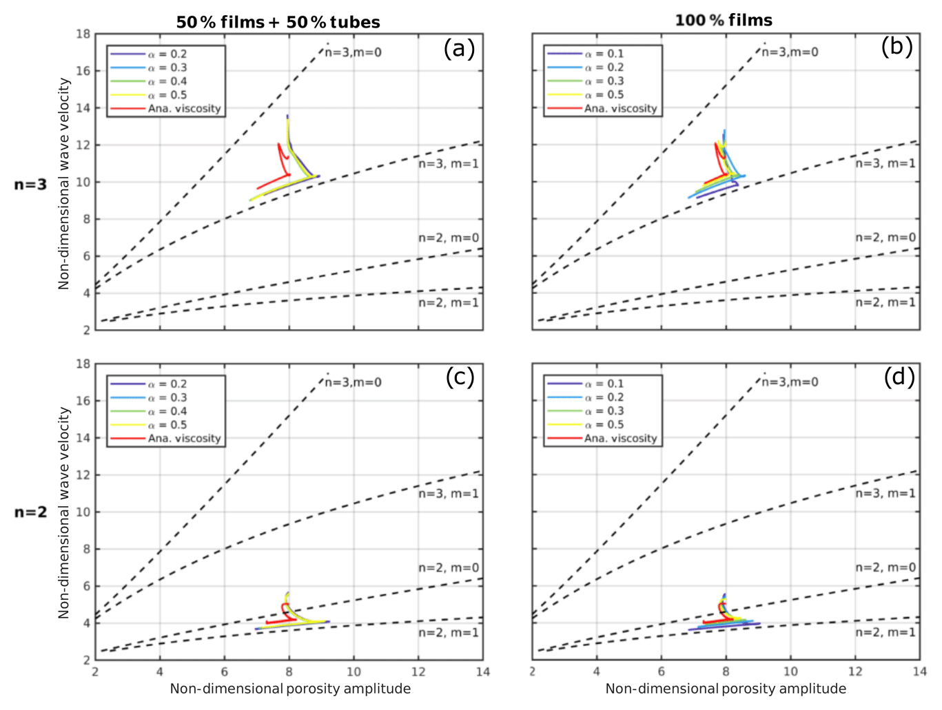
Figure 5Dispersion curves of solitary waves with (a) n=3, films and tubes; (b) n=3, films; (c) n=2, films and tubes; and (d) n=2, films for different aspect ratios.

Download

Changing n of the permeability–porosity relation to 2 decreases the wave velocities significantly (Fig. 5c, d). This drop is consistent with the simplified semi-analytical solitary wave solutions (n=2, m=1, dashed curves). In contrast to the n=3 cases, the n=2 velocities are above the Simpson and Spiegelman (2011) solutions even if the numerical 10 % overestimation is considered. As for the n=3 case, porosity waves with the stronger analytical viscosity case (Eqs. 1 and 2) are slightly faster than the new weaker viscosity cases.

While the ascending phase velocity of the wave is only slightly affected by the different viscosity laws, the width of the wave changes more strongly. In Fig. 6 the half widths of the solitary waves of amplitude of 8 are plotted against the corresponding wave velocities for the different viscosity laws. For n=2 (Fig. 6a) and 100 % films the wave gets wider for higher aspect ratios, while for the mixed geometry the widths stay more or less constant. The velocity increases only slightly with the aspect ratio. For n=3 (Fig. 6b) and 100 % films the width increases with aspect ratio, but in contrast to n=2 the phase velocity decreases with increasing aspect ratio. For the mixed geometry the velocity and half width variations are minor again. These results show that as long as melt tubes represent a significant portion of the total melt volume (here 50 %), they control the porosity wave dynamics and keep the porosity wave properties rather fixed. Only in the absence of tubes do compact melt pockets with large aspect ratios significantly broaden the waves. For the stiff case of analytical viscosity (Eqs. 1 and 2), the half width of the wave is comparable to the weaker films with aspect 0.2, but the velocities are larger (Fig. 6a, b, light-brown symbols).

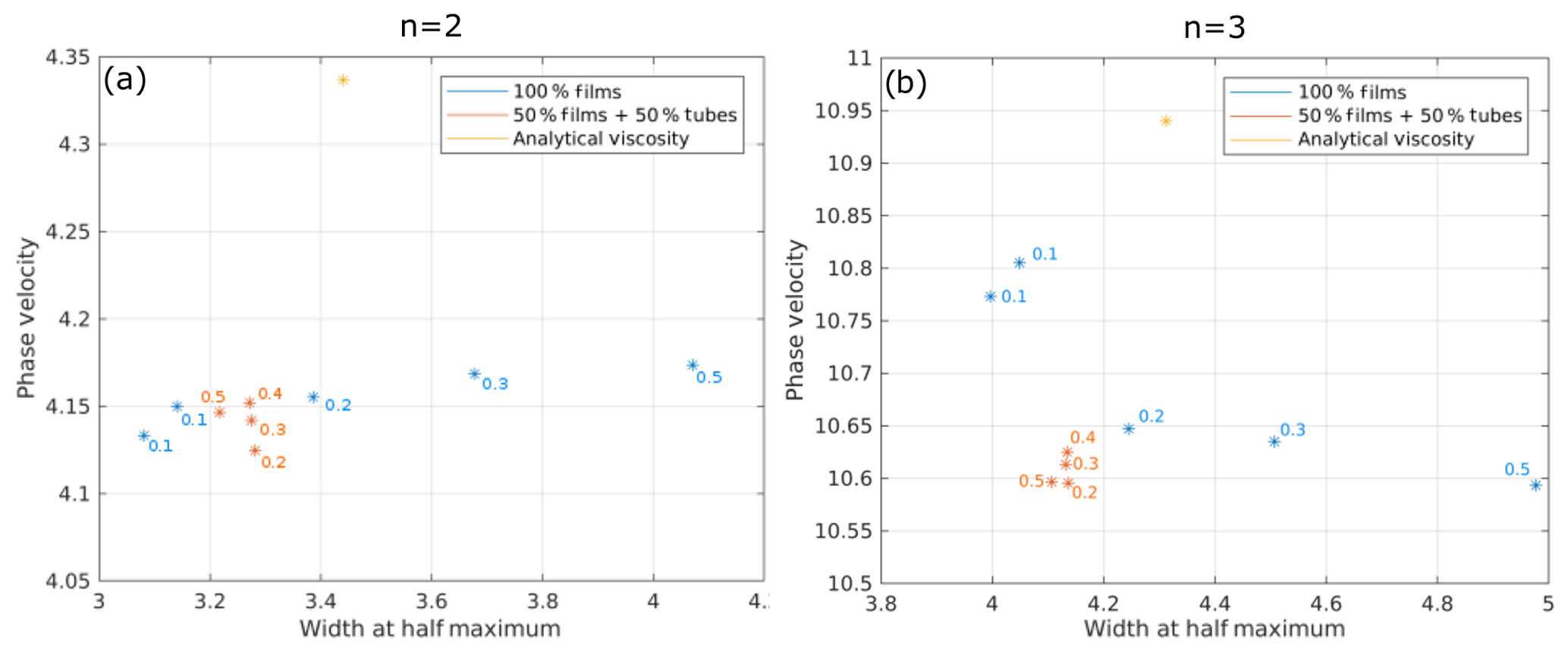
Figure 6Non-dimensional half width plotted against non-dimensional phase velocity for a porosity wave of amplitude 8 for different viscosity laws. The numbers give the aspect ratios of the films or melt pockets. The background porosity is 0.5 %. (a) Permeability–porosity exponent n=2 and (b) n=3.

Download

Another interesting phenomenon to observe is the matrix velocity in the center of the wave, which increases for all geometries with aspect ratio (Fig. 7). While for 100 % films this increase is stronger, for both geometries the velocities are approximately equal at aspect ratios between 0.2 and 0.3. For n=2 (Fig. 7a), the matrix velocities are always positive, meaning that despite a slow negative background velocity of the matrix it rises in the center of the wave (together with the melt). Interestingly, for n=3 (Fig. 7b) and small aspect ratios (0.1 and 0.2, i.e., weaker effective matrix viscosities), the direction of flow of the matrix is changed and the matrix in the center flows downwards, i.e., against the direction of melt flow. Assuming constant matrix shear and bulk viscosities, Scott (1988) observed a similar switch from negative to positive matrix velocities in the center of a 2-D solitary wave when the ratio of the bulk-to-shear viscosity was increased from 1 to 9 for n=3. We see this switch around α=0.25, corresponding to a bulk-to-shear viscosity at the center of the porosity wave of about 16, and higher elsewhere. Such a switch can be explained by an increasing role of diapiric flow, which is v₁ related, incompressible and moving upward in the center of the wave, with respect to the compaction flow, which is v₂ related, irrotational and moving downward in the center of the wave (see Eq. 12). Weakening of the bulk viscosity within the porosity wave relative to the shear viscosity allows for stronger decompaction and compaction rates, which amplify the downward compaction flow with respect to the upward diapiric flow.

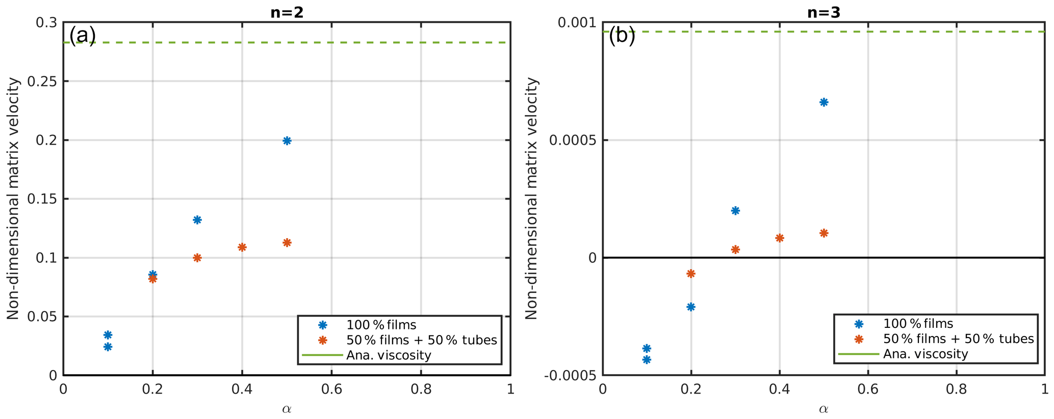
Figure 7Matrix velocity in the center of a wave with an amplitude of 8 as a function of the aspect ratio of the films for (a) n=2 and (b) n=3. The background porosity for all models was 0.005.

Download

In the previous models the scaling background porosity of 0.005 and maximum wave amplitudes of 10 to 12 imply maximum melt fractions of 5 % to 6 %. Thus, the matrix shear viscosity decrease was only small, on the order of 10 % for the aspect ratio 0.1 models and on the order of 5 % for the stiffer analytical viscosity laws (1) and (2). This explains the rather mild rheology effect when comparing the effect of the different viscosity laws. With the aim to reach higher maximum melt fractions associated with stronger rheological effects, we carried out a model series with increased background porosities, both applying the analytical viscosity law (m=1) and our weaker matrix viscosities with 100 % films with an aspect ratio 0.1 (Fig. 8). The increase in the background porosity from 0.5 % to 1.5 % has only a minor influence on the behavior of the solitary wave for models which use the analytical viscosity law (m=1): the half width of the wave is almost completely unaffected (by ∼1 %), while the phase velocity is increased by only approximately 2.5 %. Using a viscosity law based on a melt geometry consisting of 100 % films and an aspect ratio of 0.1, the differences become significant. The half width decreases to ∼70 % of its initial value, and the phase velocity decreases by up to 20 % with increasing background porosity, i.e., with an increased maximum porosity within the wave. Thus, the half widths and phase velocities show a significant difference to the analytical viscosity law (Fig. 8). In fact, the phase velocities show the opposite behavior to the analytical viscosity law (see Fig. 8b). These models suggest that the high melt fractions within the waves, which are associated with a significant local matrix weakening, both for shear and bulk viscosity, lead to effectively shortened compaction lengths within the wave, i.e., to a narrowing and focusing of the wave. Such narrower waves contain less melt than broader waves of the same amplitude, i.e., less buoyancy, which slows down the rising phase velocity.

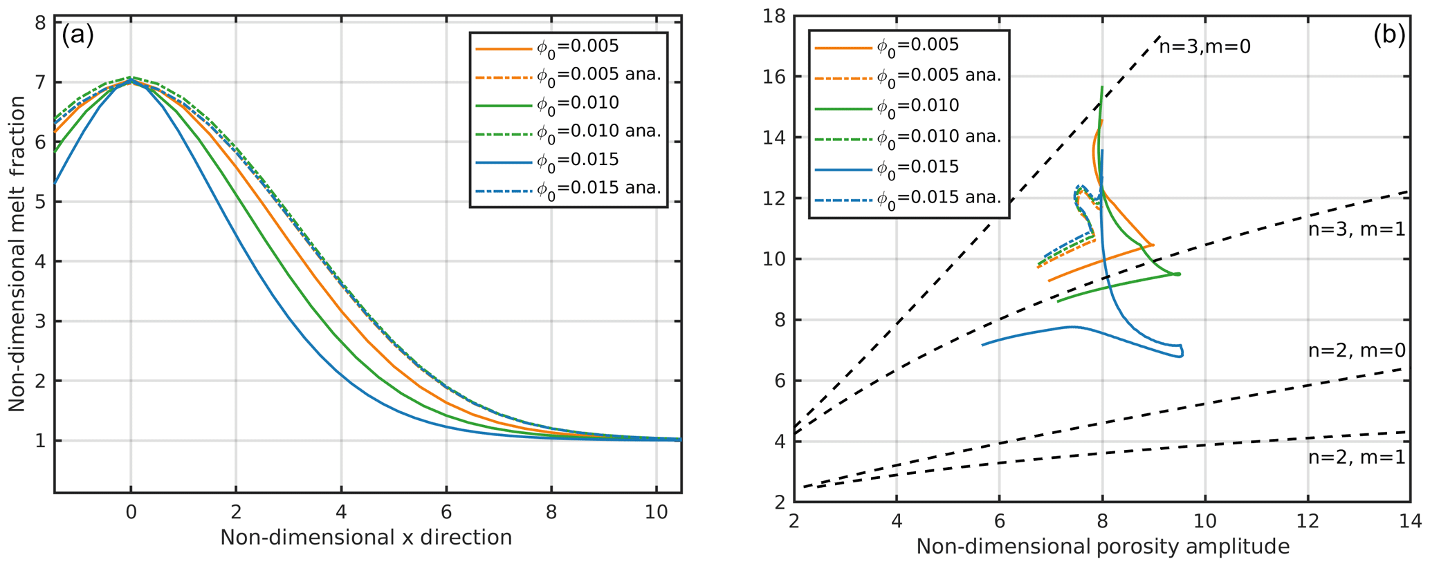
Figure 8(a) Horizontal profiles through ascending waves and (b) dispersion curves with different background porosities but the same non-dimensional amplitude of 7. The dot-dashed curves were calculated with the simplified analytical viscosity law (m=1). The solid lines were calculated with a viscosity law based on 100 % films and an aspect ratio of 0.1.

Download