Effects of finite source rupture on landslide triggering: the 2016 <i>M</i><sub>w</sub> 7.1 Kumamoto earthquake

von Specht, Sebastian; Ozturk, Ugur; Veh, Georg; Cotton, Fabrice; Korup, Oliver

doi:https://doi.org/10.5194/se-10-463-2019

Articles | Volume 10, issue 2

https://doi.org/10.5194/se-10-463-2019

Articles | Volume 10, issue 2

Research article

04 Apr 2019

Research article |

| 04 Apr 2019

Effects of finite source rupture on landslide triggering: the 2016 M_w 7.1 Kumamoto earthquake

Sebastian von Specht, Ugur Ozturk, Georg Veh, Fabrice Cotton, and Oliver Korup

Abstract

The propagation of a seismic rupture on a fault introduces spatial variations in the seismic wave field surrounding the fault. This directivity effect results in larger shaking amplitudes in the rupture propagation direction. Its seismic radiation pattern also causes amplitude variations between the strike-normal and strike-parallel components of horizontal ground motion. We investigated the landslide response to these effects during the 2016 Kumamoto earthquake (M_w 7.1) in central Kyushu (Japan). Although the distribution of some 1500 earthquake-triggered landslides as a function of rupture distance is consistent with the observed Arias intensity, the landslides were more concentrated to the northeast of the southwest–northeast striking rupture. We examined several landslide susceptibility factors: hillslope inclination, the median amplification factor (MAF) of ground shaking, lithology, land cover, and topographic wetness. None of these factors sufficiently explains the landslide distribution or orientation (aspect), although the landslide head scarps have an elevated hillslope inclination and MAF. We propose a new physics-based ground-motion model (GMM) that accounts for the seismic rupture effects, and we demonstrate that the low-frequency seismic radiation pattern is consistent with the overall landslide distribution. Its spatial pattern is influenced by the rupture directivity effect, whereas landslide aspect is influenced by amplitude variations between the fault-normal and fault-parallel motion at frequencies <2 Hz. This azimuth dependence implies that comparable landslide concentrations can occur at different distances from the rupture. This quantitative link between the prevalent landslide aspect and the low-frequency seismic radiation pattern can improve coseismic landslide hazard assessment.

Download & links

How to cite

How to cite.

Dates

Received: 21 Sep 2018 – Discussion started: 09 Oct 2018 – Revised: 15 Feb 2019 – Accepted: 27 Feb 2019 – Published: 04 Apr 2019

1 Introduction

Landslides are one of the most obvious and hazardous consequences of earthquakes. Acceleration of seismic waves alters the force balance in hillslopes and temporarily exceeds shear strength (Newmark, 1965; Dang et al., 2016). Greatly increased landslide rates have been reported on hillslopes close to earthquake rupture, mostly tied to ground acceleration (Gorum et al., 2011) and lithology (Chigira and Yagi, 2006). Substantial geomorphological and seismological data sets are required to assess the response of landslides to ground motion, and a growing number of studies have shed light on the underlying links (e.g. Lee, 2013; Allstadt et al., 2018; Roback et al., 2018; Fan et al., 2018). Several seismic measures, such as vertical and horizontal peak ground acceleration (PGA; Miles and Keefer, 2009), root-mean-square (RMS) acceleration, or Arias intensity (I_A; Arias, 1970; Keefer, 1984; Harp and Wilson, 1995; Jibson et al., 2000; Jibson, 2007; Torgoev and Havenith, 2016), seismic source-moment release, hypocentral depth, and rupture extent and propagation (Newmark, 1965), correlate with landslide density (Meunier et al., 2007).

Landslides concentrate in the area of strongest ground acceleration (Meunier et al., 2007), whereas total landslide area decreases from the earthquake rupture with the attenuation of peak ground acceleration (Dadson et al., 2004; Taylor et al., 1986). This general pattern is modified by morphometrics (e.g. local hillslope inclination and curvature) and geological parameters (e.g. lithology, geological structure, and land cover; Gorum et al., 2011; Havenith et al., 2015) that influence landslide susceptibility (Pawluszek and Borkowski, 2017) on top of seismic amplification (Maufroy et al., 2015). For instance, Tang et al. (2018) found that lithology, PGA, and distance from the rupture plane are important in assessing the distribution of landslides triggered by the 2008 Wenchuan earthquake (M_w 7.9). Fan et al. (2018) found that hillslope aspect and slope were important determinants of the landslide distribution resulting from the 2017 Jiuzhaigou earthquake (M_w 6.5).

On 16 April 2016 at 16:25 UTC central Kyushu was hit by a M_w 7.1 earthquake (Fig. 1). The left-lateral dip-slip event ruptured along the Futagawa and Hinagu faults, striking NW–SE, with a hypocentral depth of 11 km (e.g. Kubo et al., 2016). The rupture propagated northeastward and stopped at Mt Aso. Fault source inversions show a northeast propagation of the rupture originating under Kumamoto City, with highest slip near the surface at the western rim of the Aso caldera (e.g. Kubo et al., 2016; Asano and Iwata, 2016; Moore et al., 2017; Uchide et al., 2016; Yagi et al., 2016; Yoshida et al., 2017). The earthquake triggered approximately 1500 landslides (National Research Institute for Earth Science and Disaster Prevention, 2016) that concentrated mainly inside the caldera and the flanks of Mt Aso on the Pleistocene and Holocene lava flow deposits (Paudel et al., 2008; Sidle and Chigira, 2004), although most of the terrain near the earthquake rupture is rugged (Fig. 1). Thus, we hypothesize that rupture directivity causes an asymmetric distribution of landslides around the rupture plane because of more severe ground motion along the propagating rupture (Somerville et al., 1997; Hovius and Meunier, 2012). Similarly asymmetric landslide distributions attributed to rupture directivity were reported for the 2002 Denali earthquake (M_w 7.9; Frankel, 2004; Gorum et al., 2014) and the 2015 Gorkha earthquake (M_w 7.8; Roback et al., 2018). In the case of the 1999 Chi-Chi earthquake, Lee (2013) speculated that the prevalent landslide aspects were correlated to the fault movement direction (Ji et al., 2003; Meunier et al., 2008). These observations indicate that the rupture process introduces variations on the incoming energy on hillslopes.

Here we link those dominant near-surface seismic characteristics relevant to the pattern and orientation of coseismic landslides. We investigate the geological conditions (lithology, aspect, hillslope inclination, topographic amplification, and soil wetness) in central Kyushu as well as seismic waveform records from 240 seismic stations within 150 km of the rupture (Fig. 1). The two most prominent seismic effects – well founded in seismological theory (e.g. Aki and Richards, 2002) and documented in empirical relationships (e.g. Somerville et al., 1997) – are the rupture directivity and amplitude variations in fault-normal and fault-parallel motion. We examine whether the geomorphic characteristics around the Aso caldera made this area more susceptible to landslides than the surrounding topography near the earthquake rupture or whether rupture effects control the asymmetric distribution of the landslides. We introduce a ground-motion metric related to azimuth-dependent seismic energy (i.e. seismic velocity) because these effects attenuate with increasing frequency and are less captured by acceleration-based metrics. We conclude by proposing a new ground-motion model (GMM) that is consistent with the observed coseismic landslide pattern.

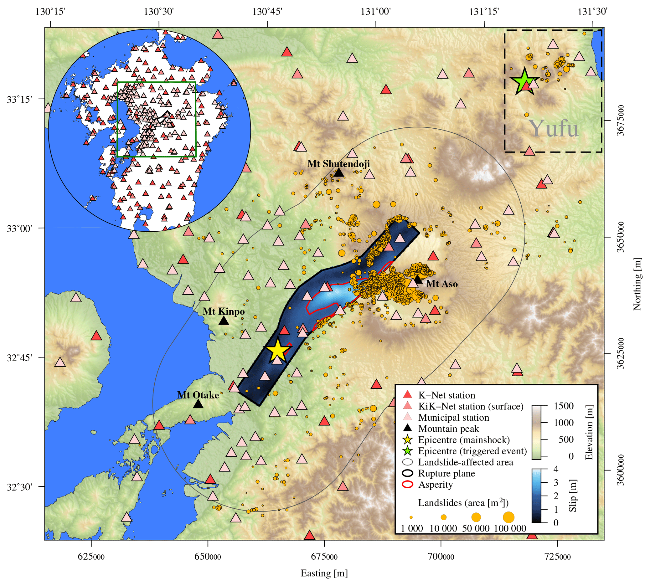
https://www.solid-earth.net/10/463/2019/se-10-463-2019-f01

Figure 1The area of Kyushu affected by coseismic landslides triggered by the 2016 M_w 7.1 Kumamoto earthquake. The coloured patch is the slip distribution of the rupture model by Kubo et al. (2016), and the dashed box encompasses landslides related to the triggered event in Yufu (epicentre location after Uchide et al. (2016)). The inset map shows the station network within 150 km of the rupture.

Download

2 Data

We combine data sets on the response of landslides to the earthquake, including topography, land cover, geology, seismic waveforms, velocity structure, near-surface characteristics, and landslide location and planform (Fig. 2).

https://www.solid-earth.net/10/463/2019/se-10-463-2019-f02

Figure 2Topographic and geological features of central Kyushu with landslides (black dots), landslide-affected area (outer black line), rupture area (inner black line), hypocentre (black diamond), and mountain peaks from Fig. 1 (triangles). (a) Hillslope inclination. (b) Median amplification factor (MAF). (c) Topographic wetness index (TWI). (d) Geology of central Kyushu. The most common geological units of the landslides are shown in (e). For the landslide-affected area the dominant geological units are in (f). (g) Land cover. Land cover in the landslide areas is shown in (h) and is shown for the entire landslide-affected area in (i).

Download

2.1 Topographic data

Most topographic data used in this study are provided by the Japan Aerospace Exploration Agency (JAXA) and its Advanced Land Observing Satellite (ALOS) project with a horizontal resolution of 1^′′ (≈30 m). This digital surface model (DSM) forms the basis for computing aspect, hillslope inclination, the median amplification factor (MAF; Maufroy et al., 2015), and the topographic wetness index (Böhner and Selige, 2006). The ALOS project also provides data on land cover, including anthropogenic influence (sealing and agriculture) and vegetation, while data on major geological units are from the Seamless Digital Geological Map of Japan (scale of 1:200 000) by the Geological Survey of Japan.

2.2 Topographic amplification of ground motion

Topographic features, such as mountains and valleys, can amplify or attenuate seismic waves (Massa et al., 2014; Maufroy et al., 2012, 2015). The largest ground-motion variations occur on hillslopes and summits, whereas variations are intermediate on narrow ridges and low on valley floors. Maufroy et al. (2015) introduced proxies for these topographic site effects, of which we use the median amplification factor (MAF), based on the topographic curvature, and the S wave velocity v_S travelling at frequency f:

\begin{matrix} (1) & MAF (f) = 8 \times 10^{- 4} \frac{v_{S}}{f} C_{S} (\frac{v_{S}}{2 f}) + 1, \end{matrix}

where $C_{S} (\frac{v_{S}}{2 f})$ is the topographic curvature convolved with a normalized smoothing kernel based on two 2-D boxcar functions as a function of v_S and f.

The curvature is estimated from the DSM (Zevenbergen and Thorne, 1987; Maufroy et al., 2015), and the seismic velocity v_S is the average S wave velocity of the uppermost 500 m from the model by Koketsu et al. (2012).

Another site effect that influences landslide potential is the local soil or groundwater content, which can be modelled for uniform conditions to the first order using the topographic wetness index (TWI) of Böhner and Selige (2006):

\begin{matrix} (2) & TWI = \log \frac{A_{c}}{\tan β}, \end{matrix}

where A_c is the upslope catchment area and β is the hillslope inclination derived from the DSM with filled sinks (Planchon and Darboux, 2001).

2.3 Ground-motion data

Ground-motion data are from the KiK-Net and K-Net of the National Research Institute for Earth Science and Disaster Prevention (NIED) of Japan. NIED operates both borehole and surface stations for KiK-Net, and we use the latter only. The Japan Meteorological Agency (JMA) also released seismic data from the municipal seismic network for the largest earthquakes of the Kumamoto sequence. In total, data from 240 stations in Kyushu are available with complete azimuthal coverage within 150 km of the earthquake rupture (Fig. 1).

The analysis of seismic waveforms is based on accelerometric data only. Both the NIED and JMA data are unprocessed, and we follow the strong motion processing guidelines of Boore and Bommer (2005). We use both acceleration and velocity in further processing and integrate the accelerograms to obtain velocity records. We correct the data with the automated baseline correction routine by Wang et al. (2011). The JMA accelerometric data further require a piecewise baseline correction prior to the displacement baseline correction due to abrupt (possibly instrument-related) jumps (Boore and Bommer, 2005; Yamada et al., 2007). We use the automated correction for baseline jumps by von Specht (2019).

An earthquake was triggered approximately 80 km to the northeast in Yufu 32 s after the Kumamoto earthquake (Fig. 1; Uchide et al., 2016). Due to the close succession of the two events, waveforms of the triggered event interfere with the coda of the Kumamoto earthquake. We taper the data to reduce signal contributions by the triggered event. The taper position is based on theoretical travel time differences between the P wave (v_P=5700 m s⁻¹) arrival of the Kumamoto earthquake and the S wave arrival (v_S=3300 m s⁻¹) of the triggered event. The respective travel paths to the stations are measured from the hypocentres. Since fewer instruments are located to the northeast and the triggered event close to the sea, less than 10 % of the data are strongly contaminated by the triggered event.

NIED hosts the rupture-plane model of Kubo et al. (2016), which describes the slip history on a curved rupture plane (based on the surface traces of the Futagawa and Hinagu faults) with a total length of 53.5 km and width of 24.0 km (Fig. 1). We use the extent and shape of the rupture plane to estimate the landslide-affected area and to define the rupture-plane distance r_rup, the shortest distance from the rupture plane. We follow the approach of Somerville et al. (1999) to identify the asperity from the rupture-plane model, which is the area with more than 1.5 times the average slip.

The underground structure in terms of seismic velocities (v_P, v_S) and density (ρ) (Koketsu et al., 2012) is available for 23 layers down to the mantle in $\approx 0.1^{\circ}$ resolution covering all of Japan; we only consider the layers of the upper 0.5 km to compute a velocity average for the MAF.

NIED provides data for the subsurface shear wave velocities (v_S30) as well as site amplification factors S_amp. Contrary to v_S by Koketsu et al. (2012), v_S30 is derived for the upper 30 m only and is more suitable for energy estimates, which require velocities at the surface (recording station). The site amplification factor S_amp describes how much seismic waves are amplified by, independent of their frequency.

2.4 Landslide data

Detailed landslide data are provided by NIED as polygons (Fig. 1), mapped from aerial imagery with sub-metre resolution at different times after the Kumamoto earthquake. The first data set contains landslides that were identified between 16 and 20 April, though the area close to the summit of Mt Aso was not covered. A second data set was collected on 29 April 2016 and covers those parts of Mt Aso that remained unmapped. However, the second data set may contain rainfall-induced landslides, since the rainy season in Kyushu starts in May (Matsumoto, 1989), and there was rainfall after the Kumamoto earthquake and landslides triggered by volcanic activity. We selectively combine the two data sets for this study, using only those landslides from the second database, which are also partly present in the first data set. We exclude any rainfall triggered landslides with this approach, though possibly omitting seismically induced landslides exclusive to the second database. However, the area in question is comparatively small to the full extent of the study area, and the missing landslides are minor in terms of their area.

Several landslides cluster ≈ 80 km to the northeast of the mainshock in the municipalities Yufu and Beppu (Fig. 1), which were hit by a triggered earthquake (Uchide et al., 2016). We hypothesize that the distant northeastern landslides were induced by this triggered event. This also explains the considerable gap in landslides (≈50 km) between Yufu and Aso (Fig. 1) in otherwise steep topography.

Apart from the special release of landslide data for the 2016 Kumamoto earthquake, NIED hosts a landslide database for all Japan (National Research Institute for Earth Science and Disaster Prevention, 2014). This database covers unspecified landslides of any origin. We extract a subset from this landslide database to compare it with the landslides triggered by the Kumamoto earthquake. Contrary to the special Kumamoto release, only the landslide deposits are mapped as polygons, whereas the scarps are mapped as lines. We manually define polygons representing the total landslide area bound by the scarp line and covering the deposit area to make both data sets comparable and because the landslide source area is generally not identical to the deposit area.

3 Total area affected by landsliding

We define the landslide-affected area, in which coseismic landsliding occurred, as the area spanned by the rupture-plane distance covering 97.5 % of the total landslide area (Harp and Wilson, 1995; Marc et al., 2017). Thus the total landslide-affected area is 3968.6 km² and is within 22.9 km distance from the rupture plane.

An M_w 7.1 event with a fault length of 53.5 km and an asperity length of 12.78 km (3 km) results in a landslide-affected area of 3914 km² (4406 km²) using parameters proposed by Marc et al. (2016). We derived the event depth of 11.1 km as the moment weighted average of the rupture model of Kubo et al. (2016). Both estimates are consistent with our area estimate. Marc et al. (2016) introduced a topographic constant, A_topo, relating the total landslide area to the area that excludes basins and inundated areas. We estimate A_topo from the ALOS land cover, finding that 97 % of all landslides occurred in areas without anthropogenic influence, i.e. land with urban and agricultural use, and water bodies. We exclude water bodies, urban areas – predominantly the metropolitan area of Kumamoto City, and rice paddies from the topographic analysis, obtaining an affected area of 3037 km², i.e. A_topo=0.68.

4 Total landslide area

Total landslide area is linked to several earthquake parameters, mostly magnitude and hypocentre or average rupture-plane depth (Keefer, 1984; Marc et al., 2016). We adopted the relation by Marc et al. (2016) to check for completeness of the total landslide area of 6.38 km². The actual total landslide failure plane is likely smaller, as the NIED data set provides the combined area of depletion and accumulation. The modal hillslope inclination is estimated at 15^∘. Instead of the earthquake magnitude scaling relation (Leonard, 2010) used by Marc et al. (2016), we use the rupture extent reported by Kubo et al. (2016). The area model requires the average length of the seismic asperities, which Marc et al. (2016) globally assumed to be 3 km. However, Somerville et al. (1999) derived a relationship of asperity sizes based on the seismic moment that results in an average asperity length of 12.78 km for the 2016 Kumamoto earthquake. This length is consistent with the asperity sizes found by Yoshida et al. (2017) for their finite rupture model. The estimated landslide area with an asperity length of 3 km results in a predicted total landslide area of 12.90 km², while with the magnitude scaled asperity size of Somerville et al. (1999), the landslide area is 3.03 km². The landslide area estimates with constant asperity length and moment-dependent asperity length differ by a factor of 2 and 0.5 from the NIED data set, respectively.

Landslide concentration is defined as landslide area per area at a given distance band (Meunier et al., 2007). For the seismic processing, we consider the rupture-plane distance r_rup based on the rupture model instead of the hypocentral distance (Meunier et al., 2007) or the Joyner–Boore distance (Harp and Wilson, 1995).

5 Ground motion and seismically induced landsliding

5.1 Coseismic landslide displacement

The sliding-block model of Newmark (1965) is widely used to estimate coseismic hillslope performance (e.g. Kramer, 1996; Jibson, 1993, 2007). The model estimates the permanent displacement on a hillslope affected by ground motion. Newmark (1965) established a relation for hillslope displacement in terms of the maximum velocity at the hillslope for a single rectangular pulse, v_max (m s⁻¹):

\begin{matrix} (3) & d_{s} = \frac{v_{\max}^{2}}{2} (\frac{1}{A a_{y}} - \frac{1}{A}), \end{matrix}

where A is the magnitude of the acceleration pulse and a_y (m s⁻²) is the yield acceleration, which is the minimum pseudostatic acceleration required to produce instability. For downslope motion along a sliding plane, a_y is related to the angle of internal friction, ϕ_f, and the hillslope inclination, δ, by

\begin{matrix} (4) & a_{y} = g (\frac{\tan ϕ_{f}}{\tan δ}) \sin δ = g (\overline{FS} - 1) \sin δ, \end{matrix}

with the average factor of safety $\overline{FS}$ . Chen et al. (2017) characterized unstable hillslopes – related to both rainfall and earthquakes – by a safety factor of FS<1.5.

An upper bound for the displacement, d_s, is based on two ground-motion parameters (Newmark, 1965; Kramer, 1996):

\begin{matrix} (5) & d_{\max} = \frac{PGA}{a_{y}} \frac{{PGV}^{2}}{a_{y}}, \end{matrix}

where PGA (m s⁻²) and PGV (m s⁻¹) are the peak ground acceleration and velocity, respectively. Thus, the coseismic hillslope performance can be characterized by velocity and acceleration. In the following sections, we derive a ground-motion model based on the acceleration-related Arias intensity and the velocity-related radiated seismic energy.

5.2 Ground-motion metrics

Though PGA is the most widely used ground-motion metric in geotechnical engineering, the Arias intensity I_A (Arias, 1970) is widely used to characterize strong ground motion for landslides:

\begin{matrix} (6) & I_{A} = \frac{π}{2 g} \int_{T_{1}}^{T_{2}} a (t)^{2} d t, \end{matrix}

where g=9.80665 m s⁻² is standard gravity and T₁ and T₂ are the times where strong ground motion starts and cedes (the acceleration a(t) has units of m s⁻² and the Arias intensity has units of m s⁻¹). The Arias intensity captures both the duration and amplitude of strong motion. Empirical relationships between I_A and d_s in terms of earthquake magnitude and epicentre distance have been developed (e.g. Bray and Travasarou, 2007; Jibson, 1993, 2007).

Since PGA and I_A are related to each other (e.g. Romeo, 2000) and the hillslope displacement depends on both velocity and acceleration (Eqs. 3 and 5), it is reasonable to characterize velocity similarly to Arias intensity. The velocity counterpart to I_A is IV2, the integrated squared velocity (Kanamori et al., 1993; Festa et al., 2008):

\begin{matrix} (7) & IV 2 = \int_{T_{1}}^{T_{2}} v (t)^{2} d t . \end{matrix}

The squared velocity is also used in radiated seismic energy estimates. The quantity j_E is the radiated energy flux of an earthquake and estimated by Choy and Cormier (1986), Kanamori et al. (1993), and Newman and Okal (1998):

\begin{matrix} (8) & j_{E} = \frac{ρ c}{S_{amp}^{2}} e^{- k r_{rup}} IV 2, \end{matrix}

where ρ and c are the density and seismic wave velocity at the recording site and S_amp is the site specific amplification factor. The distance from the rupture is given by r_rup, and k is a term for path attenuation (Anderson and Richards, 1975) and effects of transmission and reflection (Kanamori et al., 1993). The attenuation constant k is also influenced by anisotropy and structure heterogeneity (Campillo and Plantet, 1991; Bora et al., 2015). The full definition of the energy flux includes two terms for compressional waves (c=v_P) and shear waves (c=v_S). The radiated energy of an earthquake, E_S, results from the integral over the wavefront surface:

\begin{matrix} (9) & E_{S} = \iint j_{E} d A, \end{matrix}

where A is the area of the surface through which the wave passes at the recording station and represents the geometrical spreading.

The radiated seismic energy E_S describes the energy leaving the rupture area and is related to the seismic moment (Hanks and Kanamori, 1979):

\begin{matrix} (10) & E_{S} = \frac{Δ σ}{2 μ} M_{0}, \end{matrix}

where Δσ is the stress drop, μ the shear modulus, and M₀ the seismic moment. We make use of this relation when considering the magnitude-related term in the ground-motion model. Since most seismic energy is released as shear waves, we apply the shear wave velocity at the recording site (v_S) to the entire waveform, i.e. we assume that all waves arrive with velocity v_S at a site. This assumption has the advantage that it does not require a separation of the record into P and S waveforms, simplifying the computation. In Appendix Appendix B we show from a theoretical perspective that using a uniform v_S has only a small impact on the overall energy estimate. The site-specific correction term for the energy estimate $\hat{E}$ based on Eqs. (8) and (9) becomes

\begin{matrix} (11) & \hat{E} = \frac{\hat{A} ρ v_{S}}{S_{amp}^{2}} e^{- k r_{rup}} IV 2 . \end{matrix}

While E_S is the radiated seismic energy at the source, $\hat{E}$ is estimated from the velocity records at a station and only approximates E_S. Therefore, $\hat{E}$ may differ from the true and unknown radiated energy E_S (Kanamori et al., 1993). Several assumptions characterize $\hat{E}$ :

All energy is radiated as S waves in an isotropic, homogeneous medium.
Geometrical spreading is corrected for an isotropic, homogeneous medium.
Since IV2 (Eq. 7) depends on the radiation pattern, $\hat{E}$ depends on the azimuth.
Attenuation is homogeneous.
Surface waves are not considered.
Site amplification is frequency-independent.

Below, we investigate the azimuthal variation in the energy estimates to characterize the radiation pattern.

The estimated wavefront area $\hat{A}$ is related to the rupture extent and r_rup, and $\hat{A}$ corresponds to a simplified version of the wavefront area approximation by Schnabel and Bolton Seed (1973) and Shoja-Taheri and Anderson (1988):

\begin{matrix} (12) & \hat{A} = 2 W L + π r_{rup} (L + 2 W) + 2 π r_{rup}^{2} . \end{matrix}

The extent of the rupture is assumed to be rectangular with length L and width W. Equation (12) describes a cuboid with rounded corners and with only half of its surface considered because no energy flux is assumed to be transmitted above ground.

While the geometrical spreading correction is expressed analytically as the wavefront area $\hat{A}$ , we estimate the attenuation parameter k. Attenuation changes with distance, as a power law at short distances (<150 km; Anderson and Richards, 1975) and longer distances are not considered. An empirical attenuation relationship is

\begin{matrix} (13) & \ln Y = C + k r_{rup}, \end{matrix}

where Y is

\begin{matrix} (14) & Y = \frac{\hat{A} ρ v_{S}}{S_{amp}^{2}} \int_{T_{1}}^{T_{2}} IV 2, \end{matrix}

i.e. the logarithm of the energy estimate without the attenuation term $e^{- k r_{rup}}$ from Eq. (11). The dummy variable C is only used for estimating k and not in the final correction for attenuation. A distance-independent form of the Arias intensity, i.e. corrected for geometrical spreading and attenuation, is defined by

\begin{matrix} (15) & I_{A, A} = \frac{\hat{A}}{S_{amp}^{2}} e^{- k r_{rup}} I_{A}, \end{matrix}

where k is determined by Eq. (13) and setting $Y = I_{A} \hat{A}$ . The corrected Arias intensity I_A,A is the acceleration-based counterpart to $\hat{E}$ .

https://www.solid-earth.net/10/463/2019/se-10-463-2019-f03

Figure 3(a) Far-field spectrum after Brune (1970). The spectrum can be read as displacement (red), velocity (black), and acceleration (blue). (b) The squared Brune spectrum corresponds to the frequency sensitivity of velocity-based IV2 (blue) and the acceleration-based I_A (black).

Download

Low-frequency effects, like directivity, are better captured with a velocity-based metric (e.g. azimuth-dependent energy estimate) than an acceleration-based metric (Arias intensity) alone.

In terms of the Fourier transform, the sensitivity of acceleration at higher frequencies becomes apparent, as the Fourier transform of the time derivative of any function is

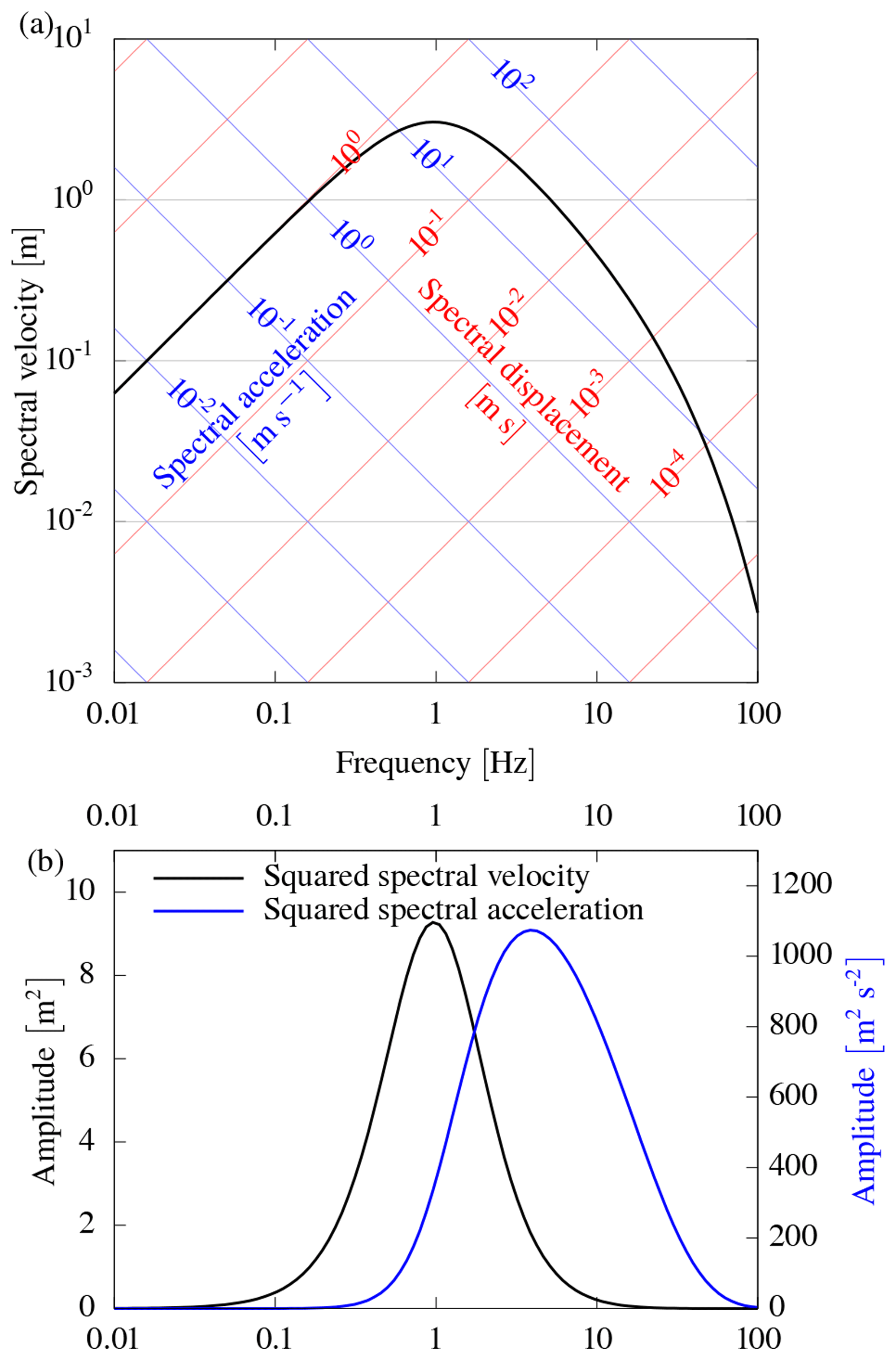
\begin{matrix} (16) & F (\dot{f} (t)) = i ω F (f (t)), \end{matrix}

and thus scales with frequency in the spectrum. The frequency sensitivity of IV2 and I_A is related to the squared spectrum given the metrics. For example, in Fig. 3 we show the different spectral sensitivities of IV2 and I_A for a theoretical seismic source spectrum (Brune, 1970). IV2, and thus $\hat{E}$ , has a higher sensitivity to lower frequencies than I_A. The low-frequency part of the spectrum can be accounted for by considering IV2 in a ground-motion model.

5.3 Landslide-related ground-motion models

The basic form of landslide-related ground-motion models for Arias intensity is based on earthquake magnitude M and distance from the earthquake rupture r (e.g. Harp and Wilson, 1995):

\begin{matrix} (17) & \ln I_{A} = p_{1} + p_{2} M + p_{3} \ln r . \end{matrix}

This form is widely used (Keefer, 1984; Harp and Wilson, 1995). In engineering seismology, ground-motion models usually have an additional distance term for anelastic attenuation:

\begin{matrix} (18) & \ln I_{A} = c_{1} + c_{2} M + c_{3} r + (c_{4} + c_{5} M) \ln . \end{matrix}

This is a modified version of the model template by Kramer (1996). While Eqs. (17) and (18) share some parameters (p₁, c₁ and p₂, c₂), the geometric spreading term includes not only distance dependence (p₃, c₄) but also has a magnitude-dependent component (c₅). In addition, anelastic attenuation is included as well (related to c₃) in Eq. (18). The template of Kramer (1996) relates to the majority of GMMs in engineering seismology. Models of this kind address strong motion in the context of landsliding (Travasarou et al., 2003; Bray and Rodriguez-Marek, 2004). The incorporation of anelastic attenuation is less common in landsliding GMMs and not mentioned in these studies but is included in more recent studies (Meunier et al., 2007, 2013; Yuan et al., 2013).

We exchange the magnitude term from Eq. (18) with a site-dependent energy term, assuming that landsliding is more related to the energy of incoming seismic waves than to the moment at the source. We replace moment magnitude by the logarithm of energy (Eq. 11), since energy is proportional to the seismic moment M₀ (Eq. 10). Based on the site-dependent energy estimate $\hat{E}$ , we propose the model

\begin{matrix} (19) & \ln I_{A} = c_{1} + c_{2} \ln \hat{E} + c_{3} r + (c_{4} + c_{5} \ln \hat{E}) \ln r . \end{matrix}

The five coefficients are inferred by non-linear least squares (e.g. Tarantola, 2005). We use the rupture-plane distance (r_rup), i.e. the shortest distance between a site and the rupture plane.

5.4 Rupture directivity model

In the NGA-west2 guidelines (Spudich et al., 2013), the directivity effect is modelled by isochrone theory (Bernard and Madariaga, 1984; Spudich and Chiou, 2008) or the azimuth between epicentre and site (Somerville et al., 1997). We use the latter approach and model directivity for estimated energy and corrected Arias intensity in a simplified way:

\begin{array}{l} (20) & \ln {\hat{E}}_{θ} = \ln {\hat{E}}_{0} + a_{E} \cos (θ - θ_{E}), \\ (21) & \ln I_{A, A, θ} = \ln I_{A, A, 0} + a_{I} \cos (θ - θ_{I}), \end{array}

where ${\hat{E}}_{0}$ and $I_{A, A, 0}$ are the offset (average), a_E and a_I the amplitude of variation with azimuth, and θ_E and θ_I are the azimuths of the maximum. The definition of θ is similar to that of Somerville et al. (1997) for the angle measured between the epicentre and the recording site, with the difference of being measured clockwise from the north. The azimuths of the maximum, θ_E and θ_I, are free parameters because (1) the rupture is assumed to have occurred on two faults and has thus variable strike and (2) the event is not pure strike-slip and has a normal faulting component. We therefore do not expect a match between the rupture strike and θ_E and θ_I. The geometrical spreading is already incorporated in the energy estimate as a distance term (Somerville et al., 1997; Spudich et al., 2013).

5.5 Model for fault-normal-to-fault-parallel ratio

The ratio of the response spectra of the horizontal sensor components is a function of oscillatory frequency f_osc.

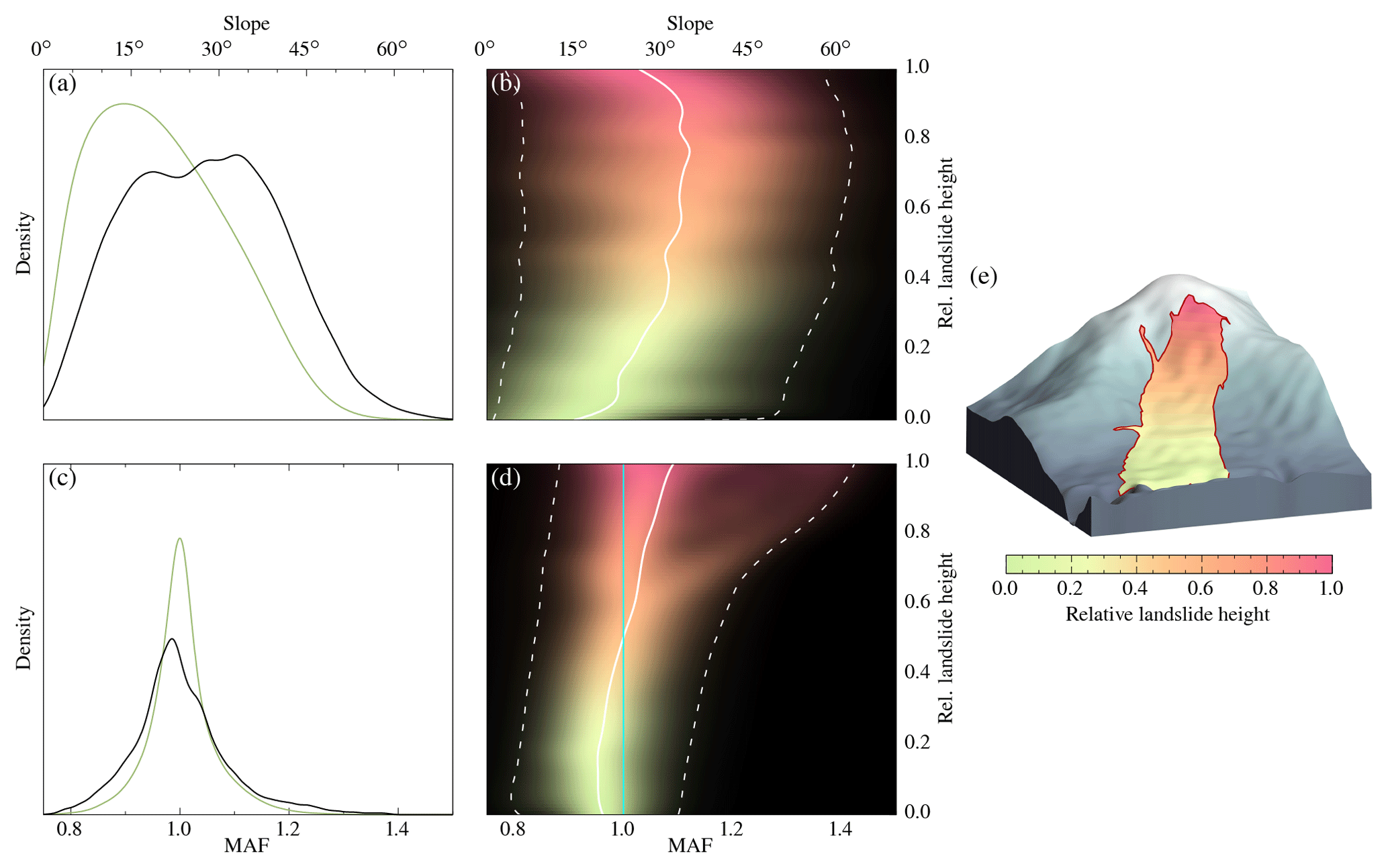
https://www.solid-earth.net/10/463/2019/se-10-463-2019-f04

Figure 4Distribution of hillslope inclination and MAF. The left column shows (a) hillslope inclinations and (c) MAF within the landslide-affected area (green) and within the landslide areas (black). The right column presents (b) hillslope inclinations and (d) MAF in different segments of the landslide areas which is expressed as relative height. Segments towards to the toe (relative height 0.0–0.5) are in green, and segments towards the crown are in red (relative height 0.5–1). The solid line is the mean, and the dashed lines enclose the 95 % uncertainty range. The concept of relative height is illustrated for the Aso Ohashi landslide in (e). MAF<1 indicates attenuation and MAF>1 amplification of seismic waves due to topography. The cyan line in (d) highlights MAF=1, i.e. no amplification or attenuation.

Download

https://www.solid-earth.net/10/463/2019/se-10-463-2019-f05

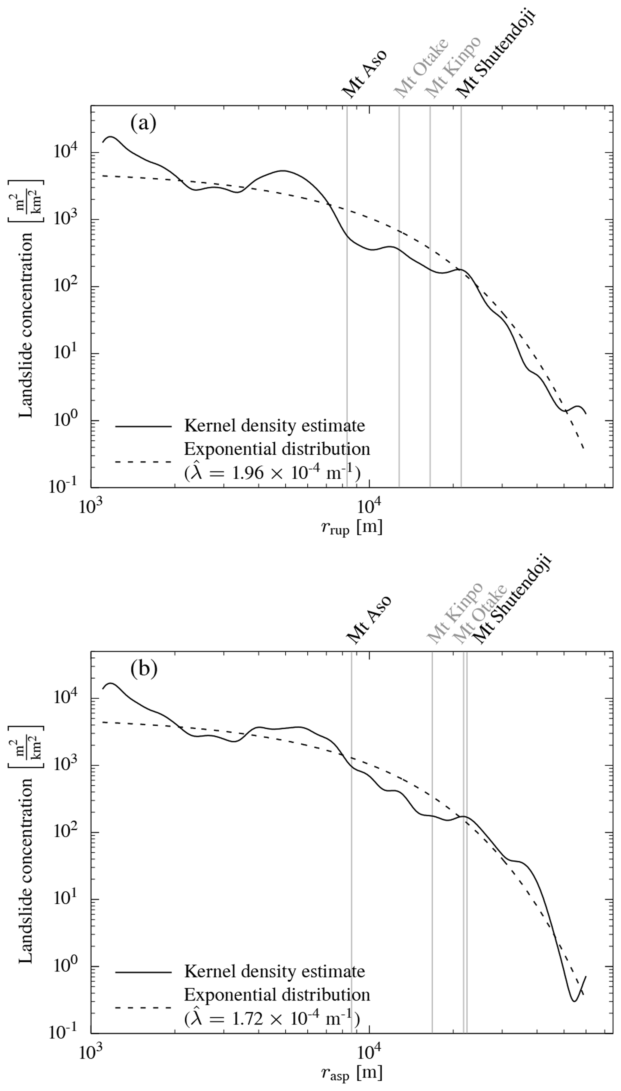
Figure 5(a) Landslide concentration with (a) rupture distance r_rup and (b) asperity distance r_asp of the Kumamoto earthquake landslides. The rate parameter of the exponentially decaying landslide concentration is estimated by maximum likelihood. The distances to the four peaks shown in Fig. 1 are given. Densities change little with distance metric, as highlighted by the similar kernel density estimates and the near-identical rate parameter estimates $\hat{λ}$ . The landslide concentration for Mt Aso depends more on the distance metric than for the other three locations. The more distant mountains have very similar concentrations despite differences in distances (in particular Mt Otake). However, when compared to Fig. 7, Mt Shutendoji has a higher landslide concentration than Mt Kinpo and Mt Otake, despite being the farthest away.

Download

https://www.solid-earth.net/10/463/2019/se-10-463-2019-f06

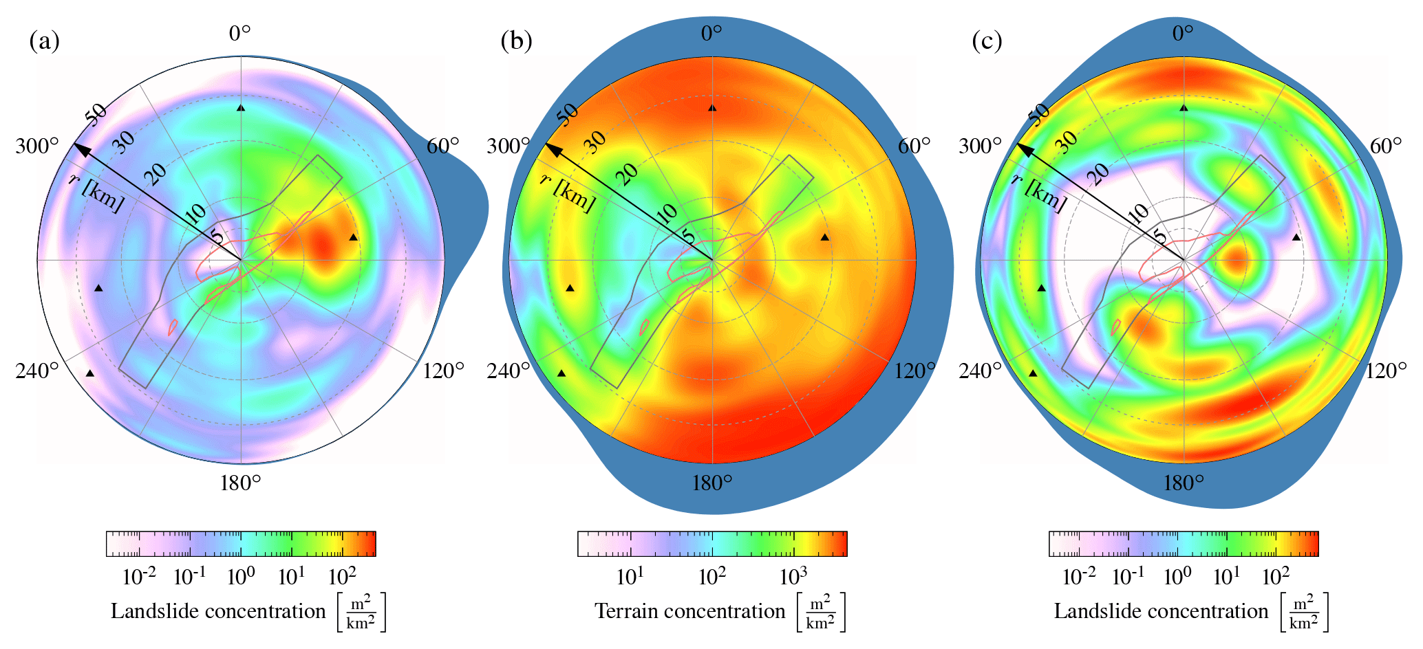
Figure 6Kernel density estimates of azimuth and distance of (a) landslide concentration of the coseismic landslides, (b) concentration of landslide-susceptible terrain with hillslope inclinations >19^∘, and (c) landslide concentration of unspecified landslides. Azimuth and distance are with respect to the asperity centroid. The marginal densities with respect to azimuth are shown in blue as outer ring. The densities are normalized to their maxima.

Download

https://www.solid-earth.net/10/463/2019/se-10-463-2019-f07

Figure 7Spatial distribution of landslides. (a) Coseismic landslides. The total landslide area at a location is shown as a colour-coded smooth function in the background; (b) same as in (a) but for unspecified landslides within the landslide-affected area of the Kumamoto earthquake.

Download

The north and east components (E, N) of the sensor are rotated to be fault-normal (FN) and fault-parallel (FP) with fault strike ϕ.

\begin{array}{l} (22) & FN = E \cos ϕ - N \sin ϕ, \\ (23) & FP = E \sin ϕ + N \cos ϕ, \\ (24) & FN / FP = \frac{{SA}_{FN} (f_{osc})}{{SA}_{FP} (f_{osc})} . \end{array}

The response spectra are calculated from accelerograms after Weber (2002), with a damping of ζ=0.05.

The amplitudes of waves parallel to rupture propagation differ from waves normal to propagation on top of the directivity effect. This variation depends on the azimuth and is larger only at high periods. The fault-normal response amplitude is larger than the fault-parallel response if directed parallel or antiparallel to the rupture. We model the ratio similar to Somerville et al. (1997):

\begin{matrix} (25) & \ln (FN / FP) = (b_{1} + b_{2} f_{osc}^{b_{3}} \cos (2 (θ - θ_{R})) H (b_{1} + b_{2} f_{osc}^{b_{3}}), \end{matrix}

where parameters b_i describe the relationship of the oscillatory frequency to the ratio, θ is the azimuth (Eq. 20), and θ_R is the azimuth of the maximal ratio. The ratio azimuth is as subject to assumptions as is its counterpart θ_E. The Heaviside function H(⋅) avoids negative values in the model, which would be equivalent to an undesired phase shift in the cosine term.

We introduced a functional form for oscillatory frequency dependence with four parameters in Eq. (20). We did not introduce a distance term and apply the model only to data with r_rup≤ 50 km.

6 Results

6.1 Topographic analysis

Landslides occurred mostly in tephra layers (Fig. 2a, b) covered by forests (Fig. 2d, e) and predominantly along the NE rupture segment. Nearly all landslides concentrated on hillslopes with a steepness between 15 and 45^∘ and an MAF ≈1 (Fig. 4a, c). Hillslope inclination and the MAF were higher towards the landslide crown (Fig. 4b, d), indicating a progressive landslide failure starting from the crown, consistent with numerical simulations by Dang et al. (2016). The TWI is linked to land cover and is highest in areas with rice paddies (Fig. 2i). Terrain with landslides has a uniformly low TWI, thus we cannot evaluate the hydrological impact on the earthquake-related landslides (e.g. Tang et al., 2018).

Most landslides originated at locations with amplified ground accelerations and steep hillslopes and ran out on flatter areas with less amplified ground acceleration. Landslides – interpreted as shear failure – start as mode II (in-plane shear) failure at the scarp and mode III (anti-plane shear) failure at the flanks (McClung, 1981; Fleming and Johnson, 1989; Martel, 2004). At later stages of the landslide rupture, mode I (widening) failure can also occur in the process (Martel, 2004). Simulations of elliptic landslides by Martel (2004) show that either the most compressive or the most tensile stresses are parallel to the major axis of the landslide, coinciding with the average landslide aspect. Yamada et al. (2013, 2018) show for several Japanese landslides that peak forces were aligned parallel to the long side of the landslides; Allstadt (2013) shows from waveform inversion for the Mt Meager landslide that force and acceleration were parallel to the long side of the landslide source area.

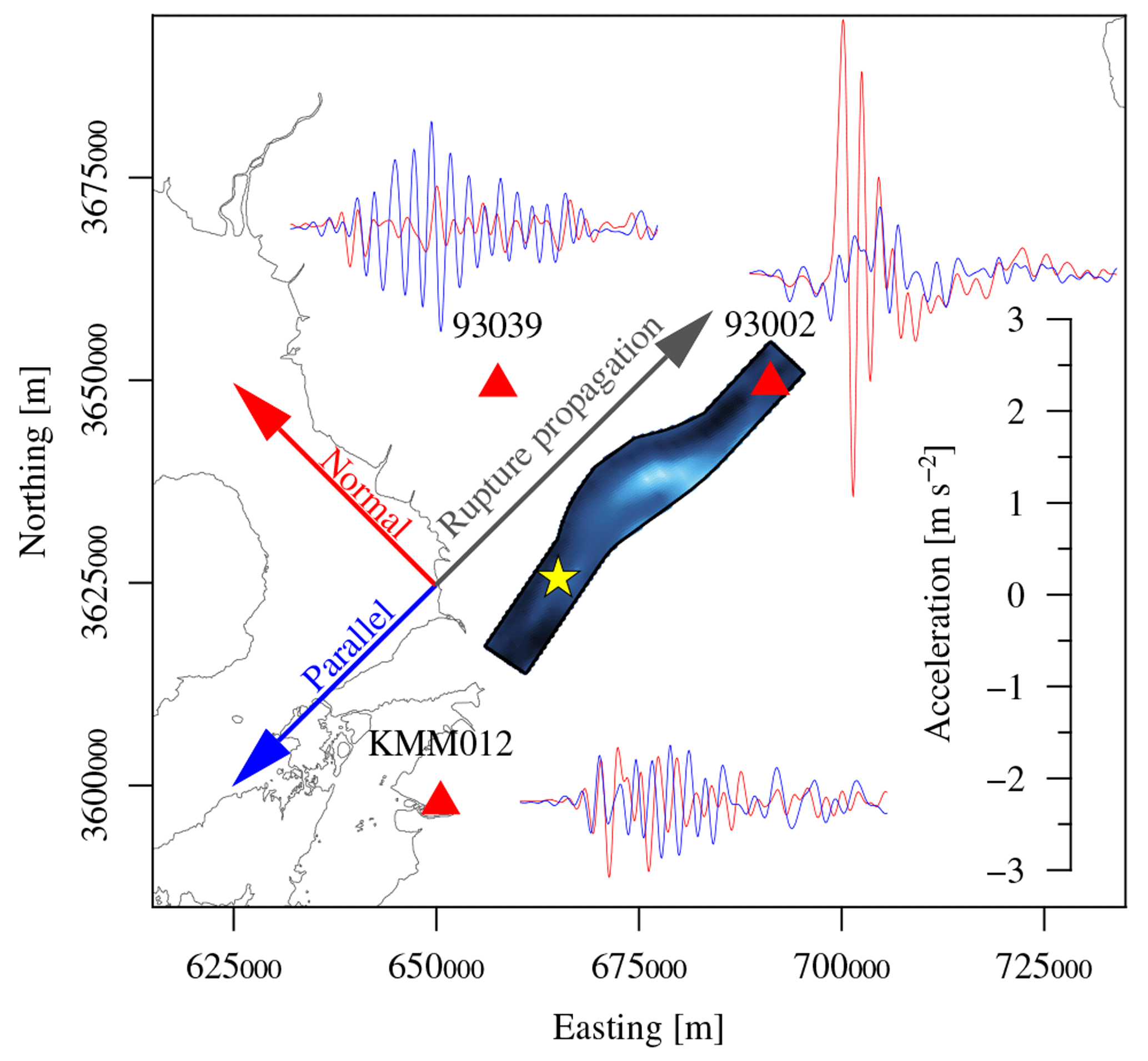
https://www.solid-earth.net/10/463/2019/se-10-463-2019-f08

Figure 8Characteristic waveforms observed in the vicinity of the rupture exhibiting rupture directivity effects. Station 93002 is in the forward-directivity region with a large amplitude pulse on the fault-normal component. Station 93039 is also in the forward-directivity region but with an offset to the rupture. In this region the fault-parallel component has higher amplitudes. The station KMM012 is in the backward-directivity region, and waveforms have longer duration without large amplitudes. The waveforms are low-pass filtered at 1.2 Hz.

Download

https://www.solid-earth.net/10/463/2019/se-10-463-2019-f09

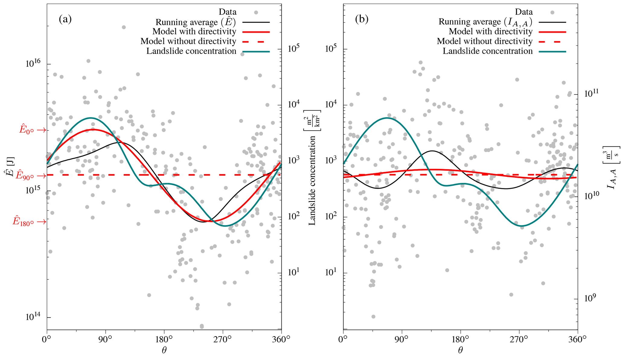
Figure 9 Energy estimates ( $\hat{E}$ ) over azimuth; (b) same as in (a) but for Arias intensity with correction for geometrical spreading (I_A,A).

Download

https://www.solid-earth.net/10/463/2019/se-10-463-2019-f10

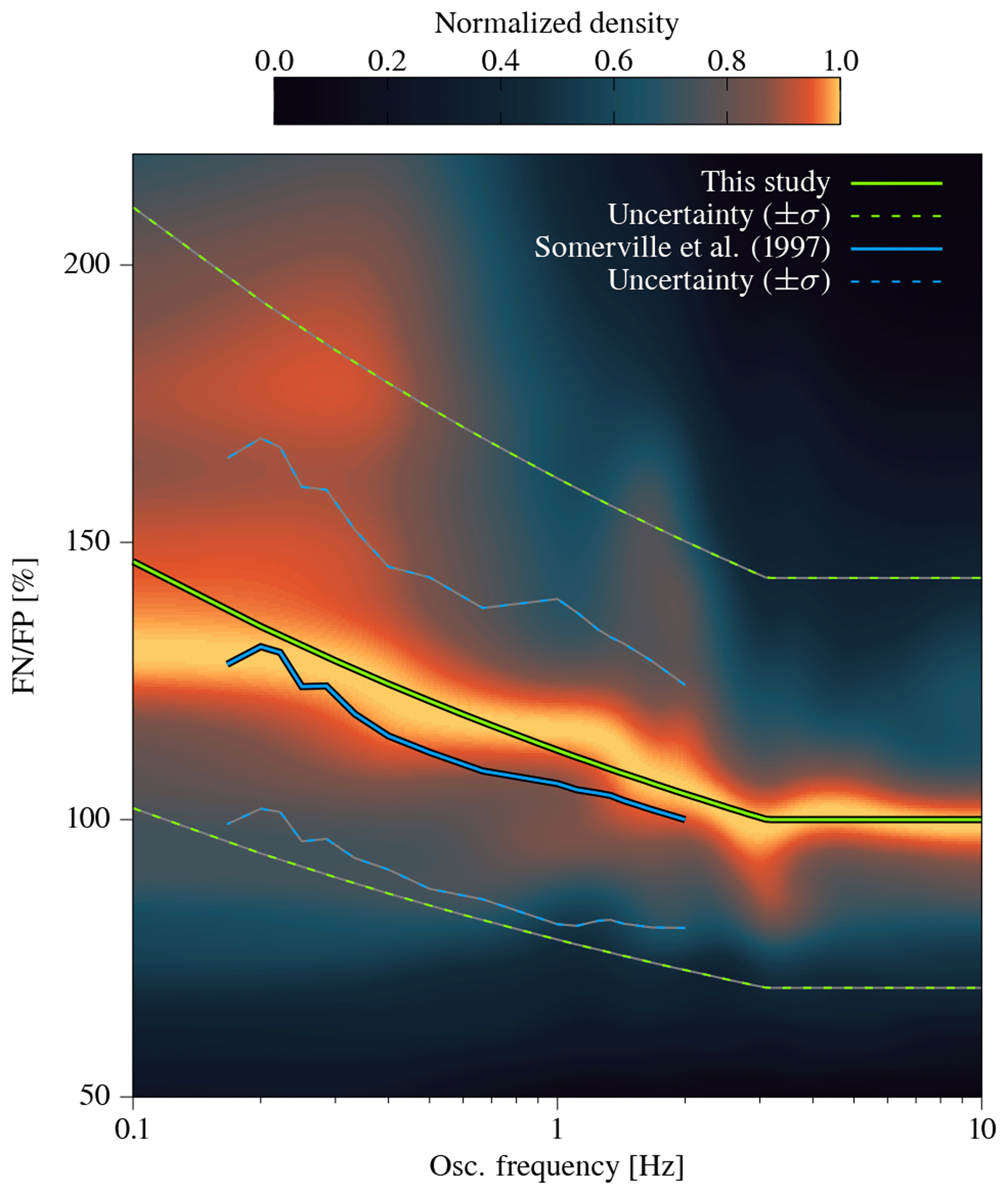
Figure 10Kernel density estimate of the amplitude ratio of response spectra of fault-normal and fault-parallel components (FN∕FP) with respect to oscillatory frequency. Beyond 2–3 Hz FN∕FP variations cease, as highlighted by our model and the model by Somerville et al. (1997).

Download

https://www.solid-earth.net/10/463/2019/se-10-463-2019-f11

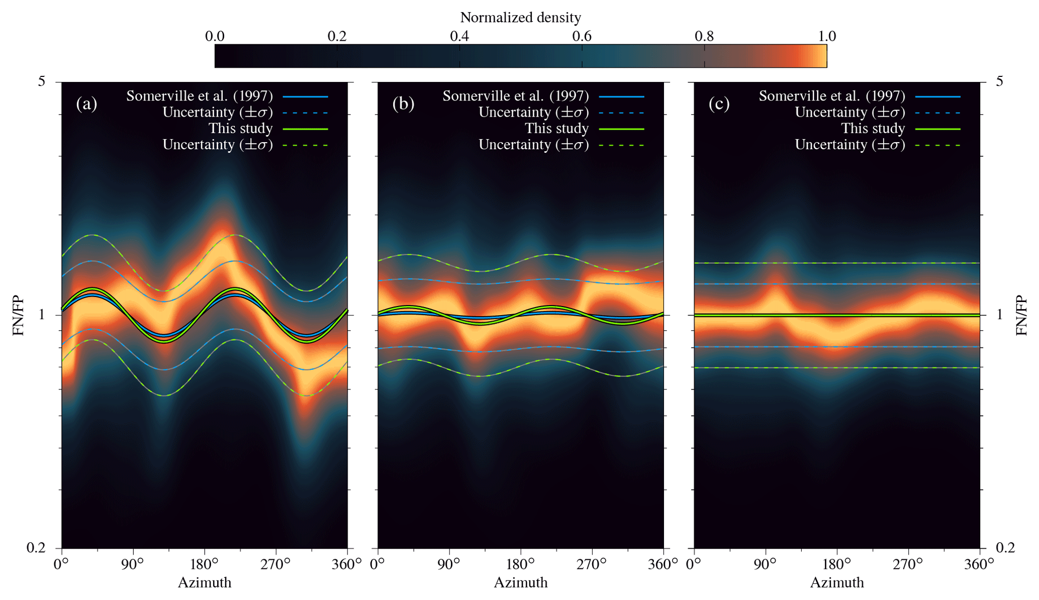
Figure 11Kernel density estimate of FN∕FP with azimuth obtained from response spectra for three different oscillatory frequency ranges: (a) 0.1–1 Hz, (b) 1.0–2.5 Hz, and (c) >2.5 Hz. For each plot, our FN∕FP model and the model by Somerville et al. (1997) are shown for (a) 0.55 Hz, (b) 1.75 Hz, and (c) 4 Hz. As in Fig. 10, amplitudes decrease with increasing oscillatory frequency.

Download

https://www.solid-earth.net/10/463/2019/se-10-463-2019-f12

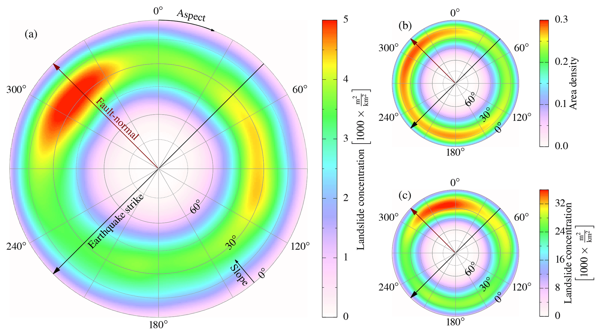
Figure 12(a) Aspect and hillslope inclination distribution within areas of the earthquake-triggered landslides. This distribution is normalized by the distribution of the aspect of all hillslopes in the landslide-affected area. The black line denotes the strike of the Kumamoto earthquake (225^∘). (b) Distribution of aspect and hillslope inclination in the landslide-affected area; (c) same as in (a) but for unspecified landslides.

Download

Mt Aso and its caldera and Mt Shutendoji had a high density of landslides (Fig. 5), whereas Mt Kinpo and Mt Otake had none, despite being closer to the epicentre and being comparably close to the rupture (Fig. 5). All these locations have comparable rock type, land cover, hillslope inclination, and MAFs. Hence, lithology, land cover, and topographic characteristics are insufficient in explaining the landslide distribution and concentration with respect to the hypocentre or the asperity.

The azimuthal density – with respect to the asperity centroid – of the unspecified landslides follows to some extent the distribution of hillslope inclinations $> 19^{\circ}$ in the landslide-affected area (Fig. 6b, c). This similarity shows that the abundance of unspecified landslides mimics the steepness of topography in the region. Densities are higher towards Mt Kinpo (W), Mt Otake (WSW), Mt Shutendoji (N), Mt Aso (E), and the Kyushu mountains (SE). The coseismic landslide distribution differs completely from the distributions of unspecified landslides and their surrounding topography (Fig. 6), respectively, as nearly all landslides happened to the northeast of the epicentre, close to the rupture plane (Fig. 7). Chen et al. (2017) identified only 29 landslide reactivations during the Kumamoto earthquake. The contrast between the distributions of unspecified landslides and earthquake-related landslides indicates a contribution by the rupture process.

6.2 Impact of finite source on ground motion and landslides

The results of the seismic analysis are given for waveforms, the basis for $\hat{E}$ and I_A, and response spectra, used for FN∕FP. To the northeast, signals with forward directivity are shorter in duration, with one or a few strong pulses (Fig. 8, top right). Waveforms with backward directivity to the southwest of the rupture are longer, with no dominant pulse (Fig. 8, bottom left). Waveforms parallel to the rupture have an intermediate duration. Waveforms in either a forward or backward direction have stronger amplitudes in the fault-normal direction, whereas waveforms outside the directivity-affected regions have stronger amplitudes in the fault-parallel direction (Fig. 8, top left).

We estimated energies $\hat{E}$ from the three-component waveforms. For the Arias intensity, both horizontal components are used. The geometrical spreading A is calculated according to Eq. (12), with a rupture length of L=53.5 km and width of W=24.0 km. Any remaining distance dependence has been corrected for by estimating and applying the attenuation parameter k (Eq. 13)

After the determination of k, $\hat{E}$ and I_A,A are considered distance-independent and can be investigated for azimuthal variations. With a reference point for the azimuth at the epicentre, $\hat{E}$ shows oscillating variations in amplitude with azimuth (Fig. 9a), while I_A,A exhibits a similar amplitude variations over the entire azimuthal range (Fig. 9b). The running average based on a von Mises kernel (κ_vM=50) of $\hat{E}$ and I_A,A shows increased $\hat{E}$ between 45 and 135^∘, i.e. approximately parallel to the strike. Minimal values of $\hat{E}$ occur in the opposite direction (200–300^∘). The running average of I_A,A has several fluctuations, but these are not as wide and large as those of $\hat{E}$ . The azimuthal variation in $\hat{E}$ indicates the rupture directivity, and the absence of large variations in I_A,A indicates that the directivity effect is only evident at lower frequencies (compare with Fig. 3).

The azimuthal variation in $\hat{E}$ and I_A,A is modelled according to Eq. (20). We estimate parameters for two scenarios:

directivity is assumed, resulting in azimuthal variations where a_E and a_I are free parameters,
directivity is not assumed, resulting in no azimuthal variations with $a_{E} = a_{I} = 0$ .

The two models are compared with the Bayesian information criterion (BIC; Schwarz, 1978) for a least-squares fit:

\begin{matrix} (26) & BIC = n \ln N + N \ln {\hat{σ}}^{2}, \end{matrix}

where n is the number of estimated parameters (n=4 for the first case and n=2 for the second case), N is the number of data, and ${\hat{σ}}^{2}$ is the variance of the model residuals. The model with the smaller BIC is preferable. The starting values of the parameters are the mean of $\hat{E}$ and I_A,A, no azimuthal variation (a_d=0), and the azimuths of the maximum of ${\hat{E}}_{θ}$ and $I_{A, A, θ}$ are set to the strike of the fault ( $θ_{E} = θ_{I} = 225^{\circ}$ ).

The directivity model for $\hat{E}$ follows the trend of the data and the running average closer than the model without directivity (Fig. 9a). According to BIC, the model with directivity is preferable (BIC $_{directivity} = - 110$ , BIC $_{no directivity} = - 11$ ). In the case of the Arias intensity, the difference in BIC between the two models is less compared to the azimuth-dependent energy (Fig. 9b). Here, the model without directivity is the preferred one (BIC_directivity=30, BIC_{no directivity}=22). In consequence, azimuthal variations in wave amplitudes and energy related to the directivity effect occur at lower frequencies.

The forward-directivity waves contain a very strong low-frequency pulse (Fig. 8). The pulse amplitude depends on the ratio of rupture and shear wave velocity and the length of the rupture (Spudich and Chiou, 2008). The forward-directivity pulse is superimposed by high-frequency signals in acceleration traces but becomes more prominent in velocity traces (Baker, 2007) due to its low-frequency nature, i.e. below 1.6 Hz (Somerville et al., 1997).

The low-frequency azimuthal variations are also reflected in the spectral response of the waveforms. Spectral accelerations of stations with r_rup≤50 km were computed from 0.1 to 5 Hz at intervals of 0.01 Hz for the fault-normal and fault-parallel component. The distribution of FN∕FP shows decreasing azimuthal variability with increasing oscillatory frequency (Fig. 11). FN∕FP is most variable with azimuth at low oscillatory frequencies (0.1–1 Hz; Fig. 11a); variations are much smaller between 1 and 2.5 Hz (Fig. 11b) and nearly absent above 2.5 Hz (Fig. 11c). This decrease with frequency is captured by the FN∕FP model (Eq. 20; Fig. 10). Since our model is an average over the covered distance, with an average rupture distance of 25.06 km, we compare it to the FN∕FP model of Somerville et al. (1997) at 25 km (Figs. 10, 11). Both models show a similar decay with frequency, with our model predicting a slightly higher FN∕FP. Therefore, the wave polarity ratio related to rupture directivity is pronounced at lower frequencies and dissipates with increasing frequency, similar to the azimuthal variations observable in energy estimates (lower frequencies) but not in Arias intensity (higher frequencies).

https://www.solid-earth.net/10/463/2019/se-10-463-2019-f13

Figure 13Orientation of horizontal peak ground acceleration for the simulated waveforms. The arrow length scales with magnitude of acceleration. The simulated rupture plane is oriented as the rupture plane of the Kumamoto earthquake (strike: 225^∘, dip: 70^∘) and of elliptic shape (grey). The upper side is denoted by the green line, and the lower half is denoted by black. The rupture process originated at the hypocentre (red dot) with circular propagation outwards (white arrow).

Download

https://www.solid-earth.net/10/463/2019/se-10-463-2019-f14

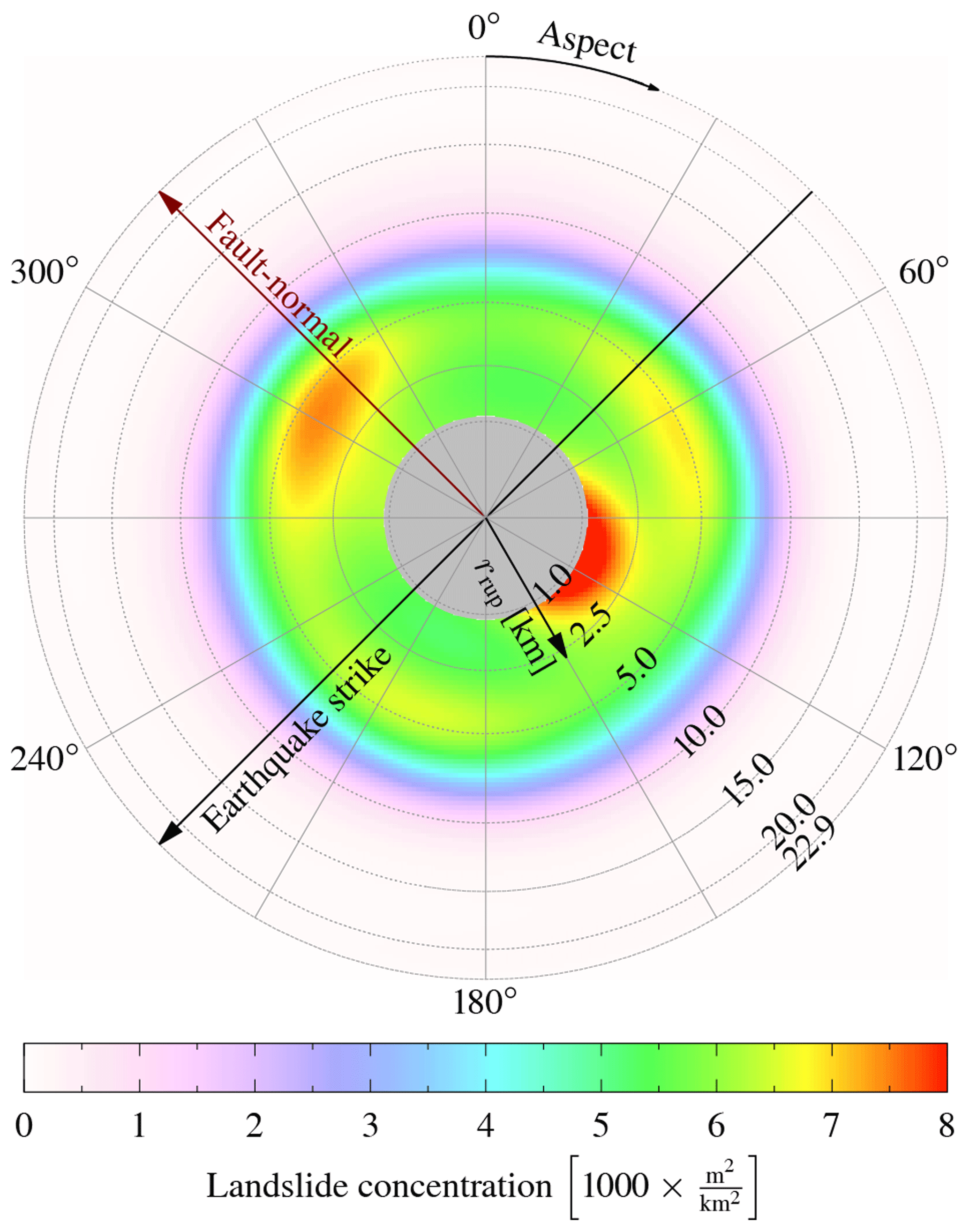
Figure 14Distribution of landslides with aspect and rupture distance. The rupture distance is measured from the model by Kubo et al. (2016). This model does not completely reach the surface, truncating distances below 1 km. The distribution has been normalized by the distribution of aspect of the affected area.

Download

https://www.solid-earth.net/10/463/2019/se-10-463-2019-f15

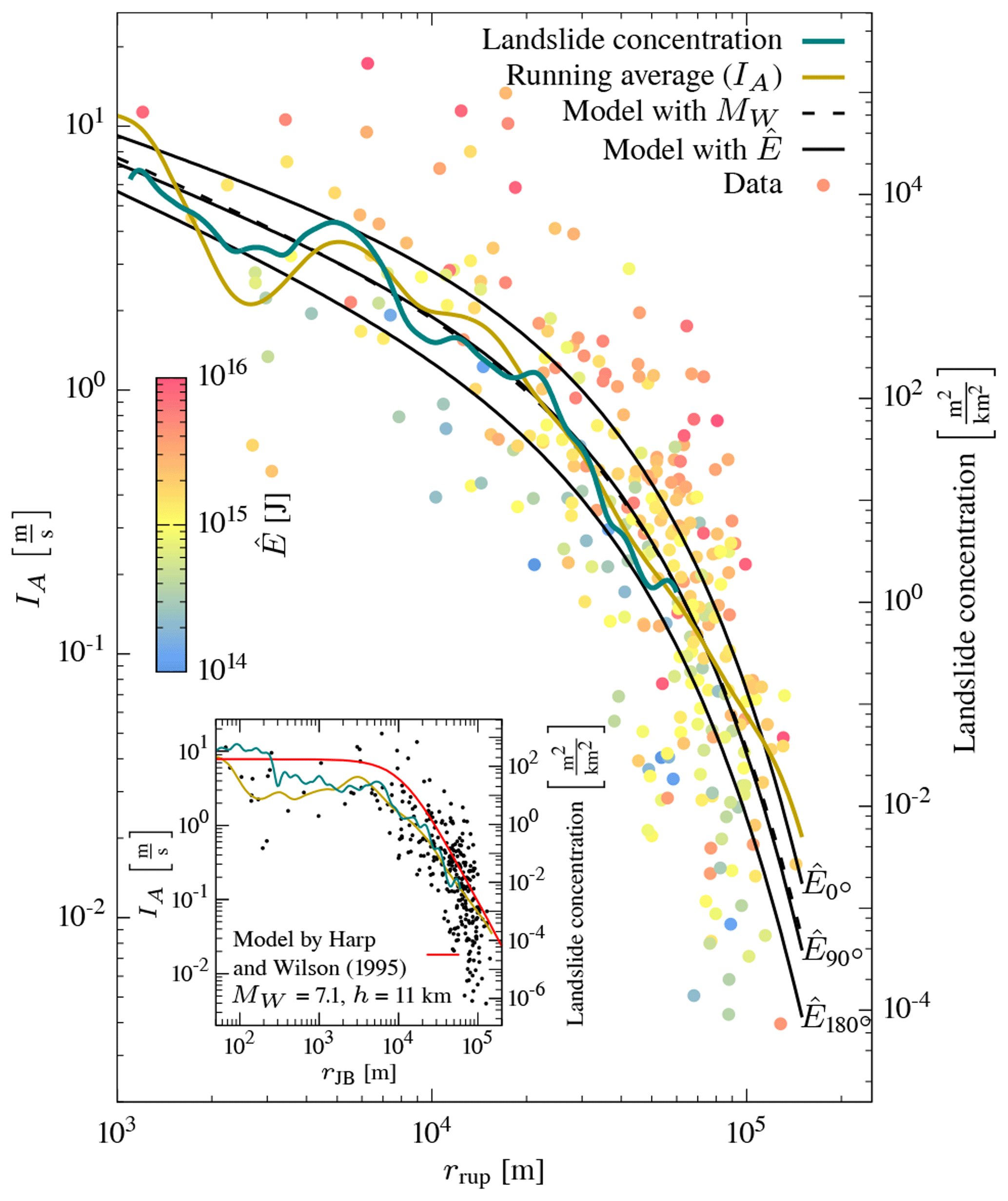
Figure 15Ground-motion model for I_A. The solid lines are the model with energy estimates for three different energy levels as in Fig. 9a. The inset figure shows, for comparison, the ground-motion model of Harp and Wilson (1995) (green) and landslide concentration density (red).

Download

The pattern of low-frequency ground motion is well reflected in that of the landslides. The azimuthal variation in $\hat{E}$ coincides with that of landslide concentration (Fig. 9). Both azimuth-dependent energy and landslide concentration have a similar trend, with the maximum being parallel to rupture direction and the minimum strike being antiparallel. The orientation of maximum FN∕FP is also reflected in the landslide aspect. The northwest and east directions show higher landslide density (Fig. 12a). The highest density of landslides has a northwestern aspect in agreement with maximum FN∕FP, both perpendicular to the strike. The eastward increased density is mostly due to landslides very close to the rupture. A look at different distances reveals that the increased density of landslides facing east by southeast is at very short distances (r_rup≤2.5 km; Fig. 14), while the northwest-facing landslides are further away ( $2.5 km < r_{rup} \leq 6$ km). Only minor landslides are farther away, with no specific pattern.

The distribution of aspect and hillslope inclination in the landslide-affected area varies little with aspect (Fig. 12b). The distinct northwest and east orientation of landslides is not an artefact of the orientation of the topography in the landslide-affected area (Fig. 12a, b). The unspecified landslides in the affected area have a near-northward aspect and deviate by $\approx 30^{\circ}$ from the earthquake-triggered landslides (Fig. 12c). This highlights that the earthquake affects landslide locations (Fig. 6) and will force failure on specific slopes facing in the direction of ground motion (Figs. 12, 14).

6.3 Ground-motion model for Kumamoto

Table 1 Parameters for ground-motion models.

Download Print Version | Download XLSX

We derived two ground-motion models for Arias intensity from data with r_rup≤150 km (Table 1; Fig. 15). One model incorporates the azimuth-dependent seismic energy (Eq. 19). The other is a conventional isotropic moment magnitude-dependent model (Eq. 18). The decay of Arias intensity with distance for both models fits the running average well and is proportional to the decrease in landslide density with distance. Variation in estimated energy is well covered by the model and spans more than 2 orders of magnitude, resulting in a variation in Arias intensity of nearly 1 order of magnitude.

The magnitude-based model is nearly equivalent to the energy-based model with $\hat{E} = 1.2 \times 10^{15}$ J. This value is close to the average energy estimate found from energy estimates of the directivity model from Eq. (20) ( $\hat{E} = 1.3 \times 10^{15}$ J). The closeness of the two values implies that the magnitude-based model can be seen as an average over the azimuth of the energy-based model.

7 Discussion

We provide a framework for characterizing coseismic landslides with an integrated approach of geomorphology and seismology, emphasizing here the role of low-frequency seismic directivity and a finite source. Given the observations of ground motion of the Kumamoto earthquake, two questions arise:

How specific is the observed ground motion, i.e. is the Kumamoto rupture particularly distinct?
As a rupture very close to the surface, how much does seismic near-field motion contribute? The second question arises because many landslides occurred very close to the rupture plane.

However, it is not possible to separate the observed waveforms into near-, intermediate-, and far-field terms. To investigate both questions, we computed theoretical waveforms after Haskell (1964), Savage (1966), and Aki and Richards (2002) from a circular rupture on an elliptic finite source with constant rupture velocity in a homogeneous, isotropic, and unbound medium (see Appendix).

Despite the simplified assumptions behind this waveform model, low-frequency ground motion captures the most prominent features of the observed waveforms. Simulated waveforms close to the rupture plane change in polarity orientation towards east–west, while a strong fault-normal polarity appears at larger distances. A decomposition into a near-field term and combined intermediate- and far-field term reveals that the former highly contributes to the ground motion at close distances. The impact of the near-field term may explain the dominance of east-facing landslides close to the rupture (Fig. 14).

The simulations also demonstrate the effect of directivity on estimates of radiated energy and Arias intensity. The azimuthal variations in simulated $\hat{E}$ are similar to the observed variations. The Arias intensity of the simulations also has azimuthal variations with the same characteristics as the energy estimate. These variations in Arias intensity are absent in the observed data, indicating that Arias intensity is more influenced by local heterogeneities and scattering than the energy estimates, as these are ignored in the simulations.

The results show that the Arias intensity is not as susceptible to the directivity effect and variations in fault-normal to fault-parallel amplitudes as the radiated energy; because of its higher sensitivity towards higher frequencies, these effects are masked by high-frequency effects such as wave scattering and a heterogeneous medium. We found that the radiation pattern related to the directivity effect is recoverable from energy estimates but not from Arias intensity. This low-frequency dependence is also seen in the response spectra ratios for FN∕FP where directivity-related amplitude variations with azimuth have been identified only for frequencies <2 Hz, in agreement with previous work (Spudich et al., 2004; Somerville et al., 1997). We introduced a modified model for Arias intensity using site-dependent seismic energy estimates instead of the source-dependent seismic magnitude to better capture the effects of low-frequency ground motion.

The conventional magnitude-based isotropic model and the azimuth-dependent seismic energy model correlate with the landslide concentration over distance (Fig. 15). As in Meunier et al. (2007) it is therefore feasible to use the ground-motion model to model the landslide concentration, P_ls(I_A), by a linear relationship:

\begin{matrix} (27) & \ln P_{ls} (I_{A}) = a_{I} + b_{I} \ln I_{A} . \end{matrix}

Azimuthal variations in landslide density correspond to azimuthal variations in seismic energy and can be described by a similar relationship:

\begin{matrix} (28) & \ln P_{ls} (E) = a_{E} + b_{E} \cos (θ - θ_{E}) . \end{matrix}

For the Kumamoto earthquake data, we estimate a_I=2.1, b_I=2.6, and $a_{E} = - 31.5$ , b_E=2.3. The azimuth-dependent landslide concentration implies similar landslide concentrations at different distances from the rupture, thus partly explaining some of the deviation in Figs. 5 and 15.

Compared to the model of Harp and Wilson (1995) (Fig. 15) our model uses rupture-plane distance, as opposed to the Joyner–Boore distance (r_JB). When using the hypocentral depth as pseudo-depth, the model of Harp and Wilson (1995) overpredicts I_A both at shorter and longer distances – irrespective of the pseudo-depth at larger distances. This misestimate is most likely due to the lack of an additional distant-dependent attenuation term in their model (Eq. 17).

The use of the MAF instead of curvature alone provides a proxy by how much a seismic wave is amplified (or attenuated) for a given wavelength and location. We show that both hillslope inclination and the MAF tend to be lower towards the landslide toe (Fig. 4). This effect is linked to the convention that landslide polygons cover both the zone of depletion and accumulation. Sato et al. (2017) consider the tephra layers rich in halloysite to be the main sliding surfaces indicating shallow landslides (Song et al., 2017). When relating coseismic landsliding to the seismic rupture, only the failure plane of the landslide matters because this is the hillslope portion that failed under seismic acceleration. Chen et al. (2017) noted, for example, that landslide susceptibility and safety factor calculation depend on whether the entire landslide or only parts – scarp area or area of dislocated mass – are considered. The reconstruction of the landslide failure planes is limited to statistical assessments of landslide inventories (Domej et al., 2017; Marc et al., 2019). However, failure may have likely originated close to the crown and then progressively propagated downward the hillslope because MAF>1 indicates an amplification of ground motion towards the crown of the landslides.

Coseismic landslide locations have a uniformly low topographic wetness index, indicating that hydrology may have added little variability to the pattern of the earthquake-triggered landslides; at least we could not trace any clear impact of soil moisture on the coseismic landslide pattern (Tang et al., 2018).

8 Conclusions

We investigated seismic waveforms and resulting landslide distribution of the 2016 Kumamoto earthquake, Japan. We demonstrate that ground motion at higher frequencies controls the isotropic (azimuth-independent) distance dependence of Arias intensity with landslide concentration. In addition, ground motion at lower frequencies influences landslide location and hillslope failure orientation, due to directivity and increased amplitudes normal to the fault, respectively. Topographic controls (hillslope inclination and the MAF) are limited predictors of coseismic landslide occurrence because areas with similar topographic and geological properties at similar distances from the rupture had widely differing landslide activity (Havenith et al., 2016; Massey et al., 2018). Nonetheless landslides concentrated only to the northeast of the earthquake rupture, while unspecified landslides have been identified throughout the affected region.

We introduced a modified model for Arias intensity using site-dependent radiated seismic energy estimates instead of the source-dependent seismic magnitude to better model low-frequency ground motion in addition to the ground motion at higher frequencies covered by the Arias intensity.

Compared to previous models widely used in landslide-related ground-motion characterization our model is based on state-of-the-art ground-motion models used in engineering seismology, which have two different distance terms, one for geometrical spreading and one for along-path attenuation. The latter is rare in landslide studies (e.g. Meunier et al., 2007; Massey et al., 2018). Our results emphasize that the attenuation term should be considered in ground-motion models, as the landslide concentration with distance mirrors such ground-motion models.

The effect of the earthquake rupture on the rupture process of the landslides results in landslide movements parallel to the strongest ground motion. Due to the surface proximity of the earthquake rupture plane, near-field ground motion influences the aspect of close landslides to be east–southeast. The intermediate- and far-field motion of the earthquake promoted more landslides on northwestern exposed hillslopes, an effect that overrides those of steepness and orientation of hillslopes in the region.

We highlight that coseismic landslide hazard estimation requires an integrated approach of both detailed ground-motion and topographic characterization. While the latter is well established for landslide hazard, ground-motion characterization has been only incorporated by simple means, i.e. without any azimuth-dependent finite rupture effects. Our results for the Kumamoto earthquake demonstrate that seismic waveforms can be reproduced by established methods from seismology. We suggest that these methods can improve landslide hazard assessment by including models for finite rupture effects.

Data availability

KiK-Net and K-Net data are accessible at http://www.kyoshin.bosai.go.jp/. The JMA special release seismic waveform data are accessible at http://www.data.jma.go.jp/svd/eqev/data/kyoshin/jishin/index.html. Coseismic landslide data are available at http://www.bosai.go.jp/mizu/dosha.html. Unspecified landslides are available at http://dil-opac.bosai.go.jp/publication/nied_tech_note/landslidemap/gis.html. The V_S30 site amplification data are available at http://www.j-shis.bosai.go.jp/map/JSHIS2/download.html?lang=en. Seismic velocities and density after Koketsu et al. (2012) are available as part of the JIVSM data set at http://www.eri.u-tokyo.ac.jp/people/hiroe/link.html. The ALOS 30 m DSM is available at https://www.eorc.jaxa.jp/ALOS/en/aw3d30/index.htm. The ALOS land use data are available at https://www.eorc.jaxa.jp/ALOS/en/lulc/lulc_index.htm. The seamless geological map of Japan is available at https://gbank.gsj.jp/seamless/download/downloadIndex_e.html. All data are free of charge, and data sources were last accessed on 19 March 2019.

Appendix A: Synthetic waveforms from displacement of a finite rupture

We illustrate the generation of ground displacement as a discontinuity across a rupture fault (e.g. Haskell, 1964, 1969; Anderson and Richards, 1975; Aki and Richards, 2002). The displacement for any point x at time t is given by

\begin{matrix} (A1) & u_{i} (x, t) = \iint_{Σ} c_{j k p q} \frac{\partial G_{i p} (D_{j} (ξ, t))}{\partial x_{q}} n_{k} d Σ, \end{matrix}

where c is the fourth-order elasticity tensor from Hooke's law, G is Green's function describing the response of the medium, D(ξ,t) is the displacement on the fault with area Σ and coordinates ξ, and n is the fault-normal vector. Summation over i, j, p, and q is implied.

While the surface integral is carried out numerically, the derivatives of Green's function for an isotropic, homogeneous, and unbound medium can be solved analytically:

\begin{array}{l} (A2) & \frac{\partial}{\partial x_{q}} G_{i p} (D_{j} (ξ, t)) = \\ \frac{15 γ_{i} γ_{p} γ_{q} - 3 (δ_{i p} γ_{q} + δ_{i q} γ_{p} + δ_{p q} γ_{i})}{4 π ρ r^{4}} \end{array}

\begin{array}{l} (A2a) & \cdot \int_{\frac{r}{α}}^{\frac{r}{β}} D_{j} (ξ t - τ) τ d τ \\ (A2b) & + \frac{6 γ_{i} γ_{p} γ_{q} - (δ_{i p} γ_{q} + δ_{i q} γ_{p} + δ_{p q} γ_{i})}{4 π ρ α^{2} r^{2}} D_{j} (ξ, t - \frac{r}{α}) \\ (A2c) & - \frac{6 γ_{i} γ_{p} γ_{q} - (2 δ_{i p} γ_{q} + δ_{i q} γ_{p} + δ_{p q} γ_{i})}{4 π ρ β^{2} r^{2}} D_{j} (ξ, t - \frac{r}{β}) \end{array}

\begin{array}{l} (A2d) & + \frac{γ_{i} γ_{p} γ_{q}}{4 π ρ α^{3} r} {\dot{D}}_{j} (ξ, t - \frac{r}{α}) \\ (A2e) & - \frac{γ_{i} γ_{p} γ_{q} - δ_{i p} γ_{q}}{4 π ρ β^{3} r} {\dot{D}}_{j} (ξ, t - \frac{r}{β}), \end{array}

where

\begin{matrix} (A3) & r = |x - ξ| and γ_{i} = \frac{x_{i} - ξ_{i}}{r}, \end{matrix}

and δ_ij is Kronecker's delta. The terms in Eq. (A2) are commonly separated into groups with respect to their distance r. In Eq. (A2) is the near-field (NF) term; as its amplitude decays with r⁻⁴, it affects the immediate vicinity of a rupture only. Terms with a distance attenuation proportional to r⁻² are called intermediate-field (IF) terms for P waves (Eq. A2a) and S waves (Eq. A2a). The remaining two terms are the far-field (FF) terms for P waves (Eq. A2b) and S waves (Eq. A2b) with a decay proportional to r⁻¹. A major difference between the NF and IF terms and the FF terms is that the former depend on the slip on the rupture, and they are the cause for static and dynamic displacement, whereas the latter are functions of the time derivative of slip and result in dynamic displacement only.

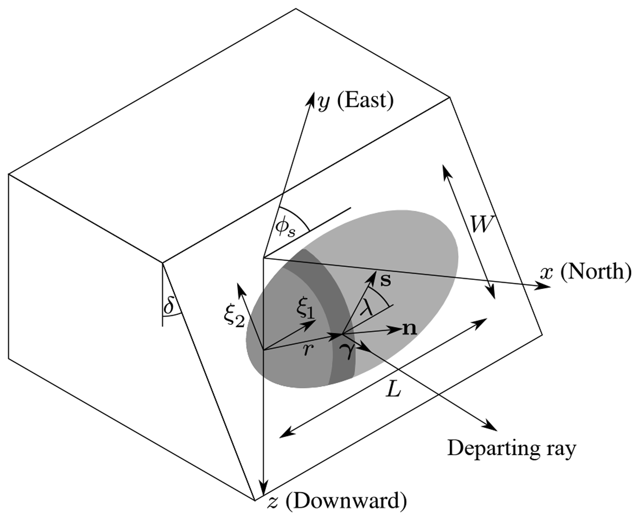
https://www.solid-earth.net/10/463/2019/se-10-463-2019-f16

Figure A1Set-up of the rupture model. Grey ellipse represents the rupture: light grey area is unruptured, medium grey area is slipping, and the dark grey area is after slip arrest.

Download

The slip function in time is related to the Yoffe function of Yoffe (1951) and Tinti et al. (2005), with rise time T. We use the slip distribution of Savage (1966) to describe the amplitude distribution of the slip on the rupture as well as the elliptical fault shape and rupture propagation from Savage (1966). The slip amplitude is given by

\begin{matrix} (A4) & D (ξ) = D_{0} \sqrt{1 - {(\frac{ξ_{1} - p ϵ \frac{L}{2}}{\frac{L}{2}})}^{2} - {(\frac{ξ_{2}}{\frac{W}{2}})}^{2}}, \end{matrix}

where D₀ is the maximum displacement at the centre of the fault, L and W are the length and width of the fault with eccentricity $ϵ = \sqrt{1 - {(\frac{W}{L})}^{2}}$ , and p determines whether the rupture starts at the focus at the front of the rupture plane (strike-parallel, p=1) or at the focus at the end (strike-antiparallel, $p = - 1$ ). The rupture originates in one of the two foci and propagates radially away from the source with constant velocity ζ and terminates when it reaches the rupture boundary. The slip vector $\hat{s}$ describes the orientation of the displacement D(ξ) on the fault plane. We follow the definition of $\hat{n}$ and $\hat{s}$ in terms of fault strike ϕ_s, dip δ, and rake λ from Aki and Richards (2002):

\begin{matrix} (A5) & \hat{n} = (\begin{array}{c} - \sin δ \sin ϕ_{s} \\ \sin δ \cos ϕ_{s} \\ - \cos δ \end{array}), \end{matrix}

\begin{matrix} (A6) & \hat{s} = (\begin{array}{c} \cos λ \cos ϕ_{s} + \cos δ \sin λ \sin ϕ_{s} \\ \cos λ \sin ϕ_{s} - \cos δ \sin λ \cos ϕ_{s} \\ - \sin λ \sin δ \end{array}) . \end{matrix}

The displacement vector D in Eq. (A2) is given by

\begin{matrix} (A7) & D = D (ξ) \hat{s} . \end{matrix}

We consider an isotropic medium, and the elasticity tensor c from Eq. (A1) is

\begin{matrix} (A8) & c_{j k p q} = δ_{j k} δ_{p q} λ_{M} + (δ_{j p} δ_{k q} + δ_{j q} δ_{k p}) μ_{M}, \end{matrix}

where λ_M and μ_M are the Lamé constants of the isotropic medium:

\begin{matrix} (A9) & λ_{M} = ρ (v_{P}^{2} + 2 μ_{M}), μ_{M} = ρ v_{S}^{2} . \end{matrix}

We set λ_M=μ_M, resulting in the widely observed relation $v_{P} = v_{S} \sqrt{3}$ .

With the assumptions outlined above it is possible to calculate the displacement of an earthquake at location x with 12 parameters (Fig. A1):

fault size and orientation, including length L, width W, strike ϕ_s, and dip δ;
material, including first and second Lamé constants λ_M and μ_M and density ρ (alternatively: compressional and shear wave velocities v_P and v_S and density ρ);
rupture and slip, including rupture velocity ζ, slip D₀, rise time T, rake λ and rupture orientation with respect to strike ϕ_s and rupture orientation parameter p.

The fault size and displacement of earthquakes are correlated with each other and are scaled to the magnitude. The number of parameters reduces to 10 (9 if the Lamé constants are equal) when scaling relations (e.g. Leonard, 2010; Strasser et al., 2010) are used in combination with the seismic moment M₀. The moment can be expressed as

\begin{matrix} (A10) & M_{0} = μ_{M} A \overline{D}, \end{matrix}

with shear modulus (second Lamé constant) μ_M, the rupture area – here an ellipse – $A = \frac{π}{4} L W$ , and average displacement $\overline{D}$ , which follows from Eq. (A3) as $\overline{D} = \frac{2}{3} D_{0}$ .

The results are not strictly comparable to observed data due to the model simplicity. The computed amplitudes will be smaller than observed values because no free surface is assumed. Assuming a free surface would nearly double the amplitudes from wave reflection as well as the amplifications from wave transmissions (from high- to low-velocity zones). Only direct waves are computed, and effects of reflections of different layers are not covered due to the isotropy and homogeneity. Corresponding waveforms – in particular surface waves – are not exhibited. However, the purpose of this model is to show (1) the general behaviour of waveforms in the vicinity of a rupture, which is dominated by direct waves, and (2) how amplitudes distribute relatively in space.

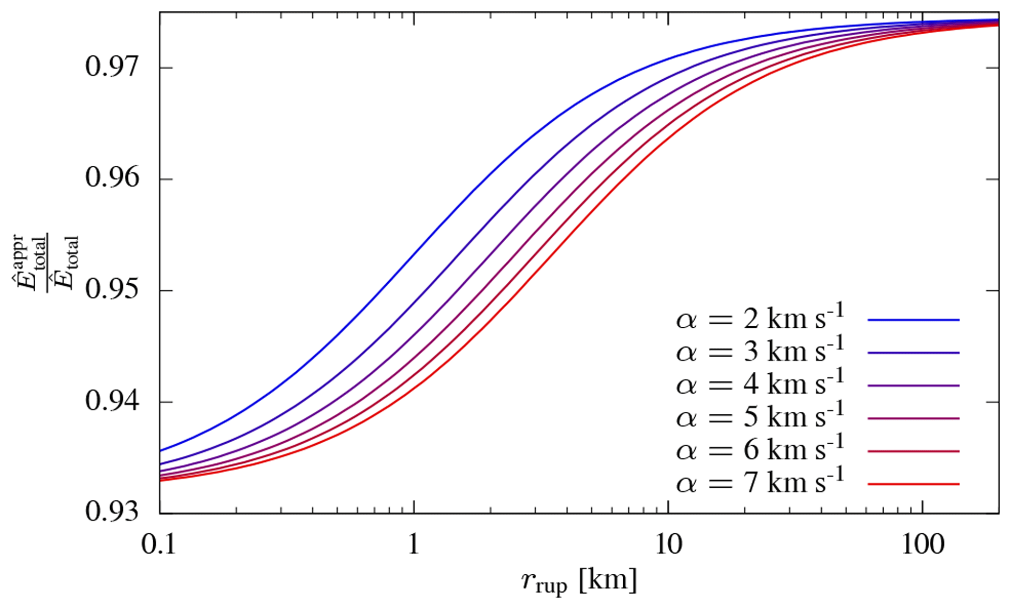
Appendix B: Radiated seismic energy estimation

https://www.solid-earth.net/10/463/2019/se-10-463-2019-f17

Figure B1Ratio between the approximate and exact energy estimates for different P wave velocities in the medium. The exact estimate assumes that P and S waves arrive at different velocities at the recording site, while the approximate estimate assumes that all waves arrive with shear wave velocity at the site. This approximation introduces only a minor underestimation, since most radiated energy is released as S waves. The distance variation arises from the different distance and velocity dependencies of the intermediate-field terms and the far-field terms.

Download

The exact calculation of radiated seismic energy is challenging. One simplifying assumption is that all waves arrive at the site with shear wave speed, which is a very good approximation for the far-field term. The reasoning can be justified from a theoretical perspective: for most earth media the ratio between the P wave velocity α and S wave velocity β is

\begin{matrix} (B1) & \frac{α}{β} = \sqrt{3} . \end{matrix}

From this and Eqs. (A2b) and (A2b), it follows that the amplitude of compressional waves is $\approx \frac{1}{{\sqrt{3}}^{3}}$ of the shear wave amplitude. If we say that the P wave train has a similar duration as the S wave train, then the energy contribution of the P waves with respect to the S waves becomes $(\frac{1}{{\sqrt{3}}^{3}})^{2} = \frac{1}{27}$ . The total energy of a signal is (Rudnicki and Freund, 1981)

\begin{matrix} (B2) & E_{total} = E_{P} + E_{S}, \end{matrix}

and can be estimated by

\begin{matrix} (B3) & {\hat{E}}_{total} = α_{S} aIV 2_{α} + β_{S} aIV 2_{β}, \end{matrix}

with the integrated squared velocity (IV2) for P and S waves from Eq. (7), the P and S wave velocities α_P and α_S at the recording site, and a constant a covering the remaining factors which are identical for both terms (compare with Eq. 8). If we express the energy contribution of P waves in terms of S waves, we can summarize the above relation to

\begin{array}{l} (B4) & {\hat{E}}_{total} = aIV 2_{β} (\frac{α_{P}}{27} + β_{S}) \\ (B5) & = aIV 2_{β} (\frac{β_{S} \sqrt{3}}{27} + β_{S}) \\ (B6) & \approx aIV 2_{β} (\frac{β_{S}}{27} + β_{S}) . \end{array}

The last expression is differs only by 2.6 % from the exact term. While slightly underestimating the energy, this approximate definition of using α_S instead of β_S does not require the identification of P and S waves. This is useful, since at short distances the S wave train is usually inseparable from the P wave train.

At shorter distances, the intermediate-field term needs also to be taken into consideration. The amplitude of the intermediate term decays with r² (Eqs. A2a, A2a), while the far-field amplitude decays with r (Eqs. A2b, A2b). That is, the amplitude scales by distance and velocities and thus the IV2 are

\begin{array}{l} (B7) & IV 2_{α} = α^{- 4} r^{- 2} {(r^{- 1} + α^{- 1})}^{2}, \\ (B8) & aIV 2_{β} = β^{- 4} r^{- 2} {(r^{- 1} + β^{- 1})}^{2} . \end{array}

Again by replacing all P wave terms by S wave terms, the total energy becomes

\begin{array}{l} (B9) & {\hat{E}}_{total} = α_{S} aIV 2_{α} + β_{S} aIV 2_{β} \\ = a r^{- 2} (α_{S} α^{- 4} {(r^{- 1} + α^{- 1})}^{2} \\ (B10) & + β_{S} β^{- 4} {(r^{- 1} + β^{- 1})}^{2}), \\ = a r^{- 2} ({\sqrt{3}}^{- 3} β_{S} β^{- 4} {(r^{- 1} + {\sqrt{3}}^{- 1} β^{- 1})}^{2} \\ (B11) & + β_{S} β^{- 4} {(r^{- 1} + β^{- 1})}^{2}) . \end{array}

With the assumption that α_S=β_S, Eq. (B4) becomes

\begin{array}{l} {\hat{E}}_{total}^{appr} \approx a r^{- 2} (β_{S} α^{- 4} {(r^{- 1} + α^{- 1})}^{2} \\ (B12) & + β_{S} β^{- 4} {(r^{- 1} + β^{- 1})}^{2}), \\ = a r^{- 2} ({\sqrt{3}}^{- 4} β_{S} β^{- 4} {(r^{- 1} + {\sqrt{3}}^{- 1} β^{- 1})}^{2} \\ (B13) & + β_{S} β^{- 4} {(r^{- 1} + β^{- 1})}^{2}) . \end{array}

The ratio between the approximation and the exact solution is

\begin{matrix} (B14) & \frac{{\hat{E}}_{total}^{appr}}{{\hat{E}}_{total}} = \frac{{\sqrt{3}}^{- 4} {(r^{- 1} + {\sqrt{3}}^{- 1} β^{- 1})}^{2} + {(r^{- 1} + β^{- 1})}^{2}}{{\sqrt{3}}^{- 3} (r^{- 1} + {\sqrt{3}}^{- 1} β^{- 1})^{2} + {(r^{- 1} + β^{- 1})}^{2}} . \end{matrix}

The two limits with respect to distance are

\begin{array}{l} (B15) & lim_{r \to 0} \frac{{\hat{E}}_{total}^{appr}}{{\hat{E}}_{total}} = \frac{{\sqrt{3}}^{- 4} + 1}{{\sqrt{3}}^{- 3} + 1} \\ (B16) & \approx 0.932, \\ (B17) & lim_{r \to \infty} \frac{{\hat{E}}_{total}^{appr}}{{\hat{E}}_{total}} = \frac{{\sqrt{3}}^{- 5} + 1}{{\sqrt{3}}^{- 6} + 1} \\ (B18) & \approx 0.974 . \end{array}

The second limit is identical to the far-field case derived above. The two limits show that even in the range of the intermediate-field term, the energy estimate deviates little when assuming that all waves arrive with β_S at the recording site. A comparison of the approximate energy estimate and the exact estimate as a function of distance and velocity is shown in Fig. B1.

Author contributions

SvS and UO devised the main conceptual ideas and performed the numerical calculations. All authors contributed to the design and implementation of the research and to the writing of the paper.

Competing interests

The authors declare that they have no conflict of interest.

Acknowledgements

We highly appreciate the help of Tomotaka Iwata and Kimiyuki Asano for providing links to additional seismic data from the municipal and NIED networks and for several helpful discussions on the specifics of the data. We are sincerely grateful to Takashi Oguchi, Yuichi Hayakawa, Hitoshi Saito, and Yasutaka Haneda for the field trip to the Aso region and fruitful discussions. We also thank Hendy Setiawan, Tao Wang, and Qiang Xu for reviewing and helping to improve the paper. Thanks to Arno Zang, John Anderson, and Odin Marc for various discussions and comments.

Sebastian von Specht, Ugur Ozturk, and Georg Veh acknowledge support from the DFG research training group “Natural Hazards and Risks in a Changing World” (grant no. GRK 2043/1). Ugur Ozturk is also supported by the Federal Ministry of Education and Research of Germany (BMBF) within the project CLIENT II – CaTeNA (FKZ 03G0878A).

The article processing charges for this open-access
publication were covered by a Research
Centre of the Helmholtz Association.

Review statement

This paper was edited by Ulrike Werban and reviewed by Hendy Setiawan, Tao Wang, and Qiang Xu.

References

Aki, K. and Richards, P. G.: Quantitative seismology, 2nd ed. University Science Books, 704 pp., 2002. a, b, c, d

Allstadt, K.: Extracting source characteristics and dynamics of the August 2010 Mount Meager landslide from broadband seismograms, J. Geophys. Res.-Earth, 118, 1472–1490, https://doi.org/10.1002/jgrf.20110, 2013. a

Allstadt, K. E., Jibson, R. W., Thompson, E. M., Massey, C. I., Wald, D. J., Godt, J. W., and Rengers, F. K.: Improving Near-Real-Time Coseismic Landslide Models: Lessons Learned from the 2016 Kaikoura, New Zealand, Earthquake, Bull. Seismol. Soc. Am., 108, 1649–1664, https://doi.org/10.1785/0120170297, 2018. a

Anderson, J. G. and Richards, P. G.: Comparison of Strong Ground Motion from Several Dislocation Models*, Geophys. J. Int., 42, 347–373, https://doi.org/10.1111/j.1365-246X.1975.tb05866.x, 1975. a, b, c

Arias, A.: Measure of earthquake intensity, Tech. rep., Massachusetts Inst. of Tech., Cambridge, Univ. of Chile, Santiago de Chile, 1970. a, b

Asano, K. and Iwata, T.: Source rupture processes of the foreshock and mainshock in the 2016 Kumamoto earthquake sequence estimated from the kinematic waveform inversion of strong motion data, Earth Planets Space, 68, 1–147, https://doi.org/10.1186/s40623-016-0519-9, 2016. a

Baker, J. W.: Quantitative Classification of Near-Fault Ground Motions Using Wavelet Analysis, Bull. Seismol. Soc. Am., 97, 1486–1501, https://doi.org/10.1785/0120060255, 2007. a

Bernard, P. and Madariaga, R.: a New Asymptotic Method for the Modeling of Near-Field Accelerograms, Bull. Seismol. Soc. Am., 74, 539–557, 1984. a

Böhner, J. and Selige, T.: Spatial prediction of soil attributes using terrain analysis and climate regionalisation, SAGA, 115, 13–27, 2006. a, b

Boore, D. M. and Bommer, J. J.: Processing of strong-motion accelerograms: Needs, options and consequences, Soil Dyn. Earthq. Eng., 25, 93–115, https://doi.org/10.1016/j.soildyn.2004.10.007, 2005. a, b

Bora, S. S., Scherbaum, F., Kuehn, N., Stafford, P., and Edwards, B.: Development of a Response Spectral Ground-Motion Prediction Equation (GMPE) for Seismic-Hazard Analysis from Empirical Fourier Spectral and Duration Models, Bull. Seismol. Soc. Am., 105, 2192–2218, https://doi.org/10.1785/0120140297, 2015. a

Bray, J. D. and Rodriguez-Marek, A.: Characterization of forward-directivity ground motions in the near-fault region, Soil Dyn. Earthq. Eng., 24, 815–828, https://doi.org/10.1016/j.soildyn.2004.05.001, 2004. a

Bray, J. D. and Travasarou, T.: Simplified Procedure for Estimating Earthquake-Induced Deviatoric Slope Displacements, J. Geotech. Geoenviron., 133, 381–392, https://doi.org/10.1061/(ASCE)1090-0241(2007)133:4(381), 2007. a

Brune, J. N.: Tectonic stress and the spectra of seismic shear waves from earthquakes, J. Geophys. Res., 75, 4997–5009, https://doi.org/10.1029/JB075i026p04997, 1970. a, b

Campillo, M. and Plantet, J.: Frequency dependence and spatial distribution of seismic attenuation in France: experimental results and possible interpretations, Phys. Earth Planet. In., 67, 48–64, https://doi.org/10.1016/0031-9201(91)90059-Q, 1991. a

Chen, C.-W., Chen, H., Wei, L.-W., Lin, G.-W., Iida, T., and Yamada, R.: Evaluating the susceptibility of landslide landforms in Japan using slope stability analysis: a case study of the 2016 Kumamoto earthquake, Landslides, 14, 1793–1801, https://doi.org/10.1007/s10346-017-0872-1, 2017. a, b, c

Chigira, M. and Yagi, H.: Geological and geomorphological characteristics of landslides triggered by the 2004 Mid Niigta prefecture earthquake in Japan, Eng. Geol., 82, 202–221, https://doi.org/10.1016/j.enggeo.2005.10.006, 2006. a

Choy, G. L. and Cormier, V. F.: Direct measurement of the mantle attenuation operator from broadband P and S Waveforms, J. Geophys. Res.-Earth, 91, 7326–7342, https://doi.org/10.1029/JB091iB07p07326, 1986. a

Dadson, S. J., Hovius, N., Chen, H., Dade, W. B., Lin, J.-C., Hsu, M.-L., Lin, C.-W., Horng, M.-J., Chen, T.-C., Milliman, J., and Stark, C. P.: Earthquake-triggered increase in sediment delivery from an active mountain belt, Geology, 32, 733–736, https://doi.org/10.1130/G20639.1, 2004. a

Dang, K., Sassa, K., Fukuoka, H., Sakai, N., Sato, Y., Takara, K., Quang, L. H., Loi, D. H., Van Tien, P., and Ha, N. D.: Mechanism of two rapid and long-runout landslides in the 16 April 2016 Kumamoto earthquake using a ring-shear apparatus and computer simulation (LS-RAPID), Landslides, 13, 1525–1534, https://doi.org/10.1007/s10346-016-0748-9, 2016. a, b

Domej, G., Bourdeau, C., Lenti, L., Martino, S., and Pluta, K.: Mean landslide geometries inferred from globla database, Ital. J. Eng. Geol. Environ., 2, 87–107, https://doi.org/10.4408/IJEGE.2017-02.O-05, 2017. a

Fan, X., Scaringi, G., Xu, Q., Zhan, W., Dai, L., Li, Y., Pei, X., Yang, Q., and Huang, R.: Coseismic landslides triggered by the 8th August 2017 Ms 7.0 Jiuzhaigou earthquake (Sichuan, China): factors controlling their spatial distribution and implications for the seismogenic blind fault identification, Landslides, 15, 967–983, https://doi.org/10.1007/s10346-018-0960-x, 2018. a, b

Festa, G., Zollo, A., and Lancieri, M.: Earthquake magnitude estimation from early radiated energy, Geophys. Res. Lett., 35, L22307, https://doi.org/10.1029/2008GL035576, 2008. a

Fleming, R. W. and Johnson, A. M.: Structures associated with strike-slip faults that bound landslide elements, Eng. Geol., 27, 39–114, https://doi.org/10.1016/0013-7952(89)90031-8, 1989. a

Frankel, A.: Rupture Process of the M 7.9 Denali Fault, Alaska, Earthquake: Subevents, Directivity, and Scaling of High-Frequency Ground Motions, Bull. Seismol. Soc. Am., 94, S234–S255, https://doi.org/10.1785/0120040612, 2004. a

Gorum, T., Fan, X., van Westen, C. J., Huang, R. Q., Xu, Q., Tang, C., and Wang, G.: Distribution pattern of earthquake-induced landslides triggered by the 12 May 2008 Wenchuan earthquake, Geomorphology, 133, 152–167, https://doi.org/10.1016/j.geomorph.2010.12.030, 2011. a, b

Gorum, T., Korup, O., van Westen, C. J., van der Meijde, M., Xu, C., and van der Meer, F. D.: Why so few? Landslides triggered by the 2002 Denali earthquake, Alaska, Quaternary Sci. Rev., 95, 80–94, https://doi.org/10.1016/j.quascirev.2014.04.032, 2014. a

Hanks, T. C. and Kanamori, H.: A moment magnitude scale, J. Geophys. Res., 84, 2348, https://doi.org/10.1029/JB084iB05p02348, 1979. a

Harp, E. L. and Wilson, R. C.: Shaking Intensity Thresholds for Rock Falls and Slides: Evidence from 1987 Whittier Narrows and Superstition Hills Earthquake Strong-Motion Records, Bull. Seismol. Soc. Am., 85, 1739–1757, 1995. a, b, c, d, e, f, g, h

Haskell, N.: Determination of earthquake energy release and ML using TERRAscope, Bull. Seismol. Soc. Am., 59, 865–908, 1969. a

Haskell, N. A.: Total energy and energy spectral density of elastic wave radiation from propagating faults, Bull. Seismol. Soc. Am., 54, 1811–1841, 1964. a, b

Havenith, H. B., Torgoev, A., Schlögel, R., Braun, A., Torgoev, I., and Ischuk, A.: Tien Shan Geohazards Database: Landslide susceptibility analysis, Geomorphology, 249, 32–43, https://doi.org/10.1016/j.geomorph.2015.03.019, 2015. a

Havenith, H.-B., Torgoev, A., Braun, A., Schlögel, R., and Micu, M.: A new classification of earthquake-induced landslide event sizes based on seismotectonic, topographic, climatic and geologic factors, Geoenviron. Disast., 3, 1–6, https://doi.org/10.1186/s40677-016-0041-1, 2016. a

Hovius, N. and Meunier, P.: Earthquake ground motion and patterns of seismically induced landsliding, in: Landslides, edited by: Clague, J. J. and Stead, D., 24–36, Cambridge University Press, Cambridge, https://doi.org/10.1017/CBO9780511740367.004, 2012. a

Ji, C., Helmberger, D. V., Wald, D. J., and Ma, K.-F.: Slip history and dynamic implications of the 1999 Chi-Chi, Taiwan, earthquake, J. Geophys. Res.-Earth, 108, 16 pp., https://doi.org/10.1029/2002JB001764, 2003. a

Jibson, R. W.: Predicting Earthquake-Induced Landslide Displacements Using Newmark's Sliding Block Analysis, Transp. Res. Rec., 1411, 9–17, 1993. a, b

Jibson, R. W.: Regression models for estimating coseismic landslide displacement, Eng. Geol., 91, 209–218, https://doi.org/10.1016/j.enggeo.2007.01.013, 2007. a, b, c

Jibson, R. W., Harp, E. L., and Michael, J. A.: A method for producing digital probabilistic seismic landslide hazard maps, Eng. Geol., 58, 271–289, https://doi.org/10.1016/S0013-7952(00)00039-9, 2000. a

Kanamori, H., Mori, J. I. M., Hauksson, E., Heaton, T. H., Hutton, K., and Jones, L. M.: Determination of Earthquake Energy Release and, Bull. Seismol. Soc. Am., 83, 330–346, 1993. a, b, c, d

Keefer, D. K.: Landslides caused by earthquakes, Geol. Soc. Am. Bull., 95, 406–421, 1984. a, b, c

Koketsu, K., Miyake, H., and Suzuki, H.: Japan Integrated Velocity Structure Model Version 1, Proceedings of the 15th World Conference on Earthquake Engineering, Lisbon, Portugal, 1–4, http://www.iitk.ac.in/nicee/wcee/article/WCEE2012_1773.pdf (last accessed: 19 March 2019), 2012. a, b, c

Kramer, S. L.: Geotechnical earthquake engineering. In prentice–Hall international series in civil engineering and engineering mechanics, Prentice-Hall, New Jersey, 1st ed. Pearson, 1996. a, b, c, d

Kubo, H., Suzuki, W., Aoi, S., and Sekiguchi, H.: Source rupture processes of the 2016 Kumamoto, Japan, earthquakes estimated from strong-motion waveforms, Earth Planets Space, 2016, 1–13, https://doi.org/10.1186/s40623-016-0536-8, 2016. a, b, c, d, e, f, g

Lee, C.-T.: Re-Evaluation of Factors Controlling Landslides Triggered by the 1999 Chi–Chi Earthquake, in: Earthquake-Induced Landslides, Springer Natural Hazards, 213–224, Springer Berlin Heidelberg, Berlin, Heidelberg, https://doi.org/10.1007/978-3-642-32238-9_22, 2013. a, b

Leonard, M.: Earthquake Fault Scaling: Self-Consistent Relating of Rupture Length, Width, Average Displacement, and Moment Release, Bull. Seismol. Soc. Am., 100, 1971–1988, https://doi.org/10.1785/0120090189, 2010. a, b

Marc, O., Hovius, N., Meunier, P., Gorum, T., and Uchida, T.: A seismologically consistent expression for the total area and volume of earthquake-triggered landsliding, J. Geophys. Res.-Earth, 121, 640–663, https://doi.org/10.1002/2015JF003732, 2016. a, b, c, d, e, f

Marc, O., Meunier, P., and Hovius, N.: Prediction of the area affected by earthquake-induced landsliding based on seismological parameters, Nat. Hazards Earth Syst. Sci., 17, 1159–1175, https://doi.org/10.5194/nhess-17-1159-2017, 2017. a

Marc, O., Behling, R., Andermann, C., Turowski, J. M., Illien, L., Roessner, S., and Hovius, N.: Long-term erosion of the Nepal Himalayas by bedrock landsliding: the role of monsoons, earthquakes and giant landslides, Earth Surf. Dynam., 7, 107–128, https://doi.org/10.5194/esurf-7-107-2019, 2019. a

Martel, S.: Mechanics of landslide initiation as a shear fracture phenomenon, Marine Geol., 203, 319–339, https://doi.org/10.1016/S0025-3227(03)00313-X, 2004. a, b, c

Massa, M., Barani, S., and Lovati, S.: Overview of topographic effects based on experimental observations: meaning, causes and possible interpretations, Geophys. J. Int., 197, 1537–1550, https://doi.org/10.1093/gji/ggt341, 2014. a

Massey, C., Townsend, D., Rathje, E., Allstadt, K. E., Lukovic, B., Kaneko, Y., Bradley, B., Wartman, J., Jibson, R. W., Petley, D. N., Horspool, N., Hamling, I., Carey, J., Cox, S., Davidson, J., Dellow, S., Godt, J. W., Holden, C., Jones, K., Kaiser, A., Little, M., Lyndsell, B., McColl, S., Morgenstern, R., Rengers, F. K., Rhoades, D., Rosser, B., Strong, D., Singeisen, C., and Villeneuve, M.: Landslides Triggered by the 14 November 2016 M_w 7.8 Kaikoura Earthquake, New Zealand, Bull. Seismol. Soc. Am., 108, 1630–1648, https://doi.org/10.1785/0120170305, 2018. a, b

Matsumoto, J.: Heavy rainfalls over East Asia, Int. J. Climatol., 9, 407–423, https://doi.org/10.1002/joc.3370090407, 1989. a

Maufroy, E., Cruz-Atienza, V. M., and Gaffet, S.: A Robust Method for Assessing 3-D Topographic Site Effects: A Case Study at the LSBB Underground Laboratory, France, Earthq. Spectra, 28, 1097–1115, https://doi.org/10.1193/1.4000050, 2012. a

Maufroy, E., Cruz-Atienza, V. M., Cotton, F., and Gaffet, S.: Frequency-scaled curvature as a proxy for topographic site-effect amplification and ground-motion variability, Bull. Seismol. Soc. Am., 105, 354–367, https://doi.org/10.1785/0120140089, 2015. a, b, c, d, e

McClung, D. M.: Fracture mechanical models of dry slab avalanche release, J. Geophys. Res.-Earth, 86, 10783–10790, https://doi.org/10.1029/JB086iB11p10783, 1981. a

Meunier, P., Hovius, N., and Haines, A. J.: Regional patterns of earthquake-triggered landslides and their relation to ground motion, Geophys. Res. Lett., 34, 1–5, https://doi.org/10.1029/2007GL031337, 2007. a, b, c, d, e, f, g

Meunier, P., Hovius, N., and Haines, J. A.: Topographic site effects and the location of earthquake induced landslides, Earth Planet. Sci. Lett., 275, 221–232, https://doi.org/10.1016/j.epsl.2008.07.020, 2008. a

Meunier, P., Uchida, T., and Hovius, N.: Landslide patterns reveal the sources of large earthquakes, Earth Planet. Sci. Lett., 363, 27–33, https://doi.org/10.1016/j.epsl.2012.12.018, 2013. a

Miles, S. B. and Keefer, D. K.: Evaluation of CAMEL - comprehensive areal model of earthquake-induced landslides, Eng. Geol., 104, 1–15, https://doi.org/10.1016/j.enggeo.2008.08.004, 2009. a

Moore, J. D. P., Yu, H., Tang, C.-H., Wang, T., Barbot, S., Peng, D., Masuti, S., Dauwels, J., Hsu, Y.-J., Lambert, V., Nanjundiah, P., Wei, S., Lindsey, E., Feng, L., and Shibazaki, B.: Imaging the distribution of transient viscosity after the 2016 M_w 7.1 Kumamoto earthquake, Science, 356, 163–167, https://doi.org/10.1126/science.aal3422, 2017. a

National Research Institute for Earth Science and Disaster Prevention: Disaster Research Institute for Science and Technology Research Materials, 1:50 000 landslide topography map, available at: http://dil-opac.bosai.go.jp/publication/nied_tech_note/landslidemap/index.html (last access: 19 March 2019), 2014. a

National Research Institute for Earth Science and Disaster Prevention: Sediment movement distribution map by the Kumamoto earthquake, available at: http://www.bosai.go.jp/mizu/dosha.html (last access: 27 June 2016), 2016. a

Newman, A. V. and Okal, E. A.: Teleseismic estimates of radiated seismic energy: The E/M 0 discriminant for tsunami earthquakes, J. Geophys. Res.-Earth, 103, 26885–26898, https://doi.org/10.1029/98JB02236, 1998. a

Newmark, N. M.: Effects of Earthquakes on Dams and Embankments, Géotechnique, 15, 139–160, https://doi.org/10.1680/geot.1965.15.2.139, 1965. a, b, c, d, e

Paudel, P. P., Omura, H., Kubota, T., and Devkota, B.: Characterization of terrain surface and mechanisms of shallow landsliding in upper Kurokawa watershed, Mt Aso, western Japan, Bull. Eng. Geol. Environ., 67, 87–95, https://doi.org/10.1007/s10064-007-0108-z, 2008. a

Pawluszek, K. and Borkowski, A.: Impact of DEM-derived factors and analytical hierarchy process on landslide susceptibility mapping in the region of Rożnów Lake, Poland, Nat. Hazards, 86, 919–952, https://doi.org/10.1007/s11069-016-2725-y, 2017. a

Planchon, O. and Darboux, F.: A fast, simple and versatile algorithm to fill the depressions of digital elevation models, CATENA, 46, 159–176, https://doi.org/10.1016/S0341-8162(01)00164-3, 2001. a

Roback, K., Clark, M. K., West, A. J., Zekkos, D., Li, G., Gallen, S. F., Chamlagain, D., and Godt, J. W.: The size, distribution, and mobility of landslides caused by the 2015 M_w 7.8 Gorkha earthquake, Nepal, Geomorphology, 301, 121–138, https://doi.org/10.1016/j.geomorph.2017.01.030, 2018. a, b

Romeo, R.: Seismically induced landslide displacements: A predictive model, Eng. Geol., 58, 337–351, https://doi.org/10.1016/S0013-7952(00)00042-9, 2000. a

Rudnicki, J. W. and Freund, L. B.: On energy radiation from seismic sources, Bull. Seismol. Soc. Am., 71, 583–595, 1981. a

Sato, T., Chigira, M., and Matsushi, Y.: Topographic and Geological Features of Landslides Induced by the 2016 Kumamoto Earthquake in the Western Part of the Aso Caldera, DPRI Ann., 60B, 431–452, 2017. a

Savage, J. C.: Radiation from a realistic model of faulting, Bull. Seismol. Soc. Am., 56, 577–592, 1966. a, b, c

Schnabel, P. B. and Bolton Seed, H.: Accelerations in rock for earthquakes in the western United States, Bull. Seismol. Soc. Am., 63, 501–516, 1973. a

Schwarz, G.: Estimating the Dimension of a Model, Ann. Stat., 6, 461–464, https://doi.org/10.1214/aos/1176344136, 1978. a

Shoja-Taheri, B. Y. J. and Anderson, J. G.: The 1978 Tabas, Iran, earthquake: an interpretation of the strong motion records, Bull. Seismol. Soc. Am., 78, 142–171, 1988. a

Sidle, R. C. and Chigira, M.: Landslides and debris flows strike kyushu, japan, Eos, 85, 145–156, https://doi.org/10.1029/2004EO150001, 2004. a

Somerville, P., Irikura, K., Graves, R., Sawada, S., Wald, D., Abrahamson, N., Iwasaki, Y., Kagawa, T., Smith, N., and Kowada, A.: Characterizing Crustal Earthquake Slip Models for the Prediction of Strong Ground Motion, Seismol. Res. Lett., 70, 59–80, https://doi.org/10.1785/gssrl.70.1.59, 1999. a, b, c

Somerville, P. G., Smith, N. F., Graves, R. W., and Abrahamson, N. a.: Modification of Empirical Strong Ground Motion Attenuation Relations to Include the Amplitude and Duration Effects of Rupture Directivity, Seismol. Res. Lett., 68, 199–222, https://doi.org/10.1785/gssrl.68.1.199, 1997. a, b, c, d, e, f, g, h, i, j, k

Song, K., Wang, F., Dai, Z., Iio, A., Osaka, O., and Sakata, S.: Geological characteristics of landslides triggered by the 2016 Kumamoto earthquake in Mt. Aso volcano, Japan, Bull. Eng. Geol. Environ., 78, 1–10, https://doi.org/10.1007/s10064-017-1097-1, 2017. a

Spudich, B. P., Chiou, B. S. J., Graves, R., Collins, N., and Somerville, P.: A Formulation of Directivity for Earthquake Sources Using Isochrone Theory, U.S. Geol. Surv. Open-File Rept. 2004-1268, p. 54, 2004. a

Spudich, P. and Chiou, B. S. J.: Directivity in NGA earthquake ground motions: Analysis using isochrone theory, Earthq. Spectra, 24, 279–298, https://doi.org/10.1193/1.2928225, 2008. a, b

Spudich, P., Bayless, J., Baker, J., Chiou, B. S. J., Rowshandel, B., Shahi, S., and Somerville, P.: Final Report of the NGA-West2 Directivity Working Group, Tech. Rep. Final, Pacific Earthquake Engineering Research Center, 2013. a, b

Strasser, F. O., Arango, M. C., and Bommer, J. J.: Scaling of the Source Dimensions of Interface and Intraslab Subduction-zone Earthquakes with Moment Magnitude, Seismol. Res. Lett., 81, 941–950, https://doi.org/10.1785/gssrl.81.6.941, 2010. a

Tang, R., Fan, X., Scaringi, G., Xu, Q., van Westen, C. J., Ren, J., and Havenith, H.-B.: Distinctive controls on the distribution of river-damming and non-damming landslides induced by the 2008 Wenchuan earthquake, Bull. Eng. Geol. Environ., 1–19, https://doi.org/10.1007/s10064-018-1381-8, 2018. a, b, c

Tarantola, A.: Inverse problem theory and methods for model parameter estimation, SIAM, 342 pp., 2005. a

Taylor, S. R., Bonner, B. P., and Zandt, G.: Attenuation and scattering of broadband P and S waves across North America, J. Geophys. Res.-Earth, 91, 7309–7325, https://doi.org/10.1029/JB091iB07p07309, 1986. a

Tinti, E., Fukuyama, E., Piatanesi, A., and Cocco, M.: A Kinematic Source-Time Function Compatible with Earthquake Dynamics, Bull. Seismol. Soc. Am., 95, 1211–1223, https://doi.org/10.1785/0120040177, 2005. a

Torgoev, A. and Havenith, H. B.: 2D dynamic studies combined with the surface curvature analysis to predict Arias Intensity amplification, J. Seismol., 20, 711–731, https://doi.org/10.1007/s10950-016-9553-0, 2016. a

Travasarou, T., Bray, J. D., and Abrahamson, N. A.: Empirical attenuation relationship for Arias Intensity, Earthq. Eng. Struct. D., 32, 1133–1155, https://doi.org/10.1002/eqe.270, 2003. a

Uchide, T., Horikawa, H., Nakai, M., Matsushita, R., Shigematsu, N., Ando, R., and Imanishi, K.: The 2016 Kumamoto–Oita earthquake sequence: aftershock seismicity gap and dynamic triggering in volcanic areas, Earth Planets Space, 68, 180 pp., https://doi.org/10.1186/s40623-016-0556-4, 2016. a, b, c, d

Wang, R., Schurr, B., Milkereit, C., Shao, Z., and Jin, M.: An Improved Automatic Scheme for Empirical Baseline Correction of Digital Strong-Motion Records, Bull. Seismol. Soc. Am., 101, 2029–2044, https://doi.org/10.1785/0120110039, 2011. a

Weber, B.: Tragwerksdynamik: Vorlesung, Sommersemester 2002, ETH Zürich, Abteilung für Bauingenieurwesen, Institut für Baustatik und Konstruktion, 170 pp., https://doi.org/10.3929/ethz-a-004375919, 2002. a

Yagi, Y., Okuwaki, R., Enescu, B., Kasahara, A., Miyakawa, A., and Otsubo, M.: Rupture process of the 2016 Kumamoto earthquake in relation to the thermal structure around Aso volcano, Earth Planets Space, 68, 118 pp., https://doi.org/10.1186/s40623-016-0492-3, 2016. a

Yamada, M., Heaton, T., and Beck, J.: Real-Time Estimation of Fault Rupture Extent Using Near-Source versus Far-Source Classification, Bull. Seismol. Soc. Am., 97, 1890–1910, https://doi.org/10.1785/0120060243, 2007. a

Yamada, M., Kumagai, H., Matsushi, Y., and Matsuzawa, T.: Dynamic landslide processes revealed by broadband seismic records, Geophys. Res. Lett., 40, 2998–3002, https://doi.org/10.1002/grl.50437, 2013. a

Yamada, M., Mangeney, A., Matsushi, Y., and Matsuzawa, T.: Estimation of dynamic friction and movement history of large landslides, Landslides, 15, 1–12, https://doi.org/10.1007/s10346-018-1002-4, 2018. a

Yoffe, E. H.: LXXV. The moving griffith crack, The London, Edinburgh, and Dublin Philosophical Magazine and Journal of Science, 42, 739–750, https://doi.org/10.1080/14786445108561302, 1951. a

Yoshida, K., Miyakoshi, K., Somei, K., and Irikura, K.: Source process of the 2016 Kumamoto earthquake (Mj7.3) inferred from kinematic inversion of strong-motion records, Earth Planets Space, 69, 64 pp., https://doi.org/10.1186/s40623-017-0649-8, 2017. a, b

Yuan, R.-M., Deng, Q.-H., Cunningham, D., Xu, C., Xu, X.-W., and Chang, C.-P.: Density Distribution of Landslides Triggered by the 2008 Wenchuan Earthquake and their Relationships to Peak Ground Acceleration, Bull. Seismol. Soc. Am., 103, 2344–2355, https://doi.org/10.1785/0120110233, 2013. a

Zevenbergen, L. W. and Thorne, C. R.: Quantitative analysis of land surface topography, Earth Surf. Proc. Land., 12, 47–56, https://doi.org/10.1002/esp.3290120107, 1987. a

Articles

Short summary

We show the landslide response to the 2016 Kumamoto earthquake (M_w 7.1) in central Kyushu (Japan). Landslides are concentrated to the northeast of the rupture, coinciding with the propagation direction of the earthquake. This azimuthal variation in the landslide concentration is linked to the seismic rupture process itself and not to classical landslide susceptibility factors. We propose a new ground-motion model that links the seismic radiation pattern with the landslide distribution.

Effects of finite source rupture on landslide triggering: the 2016 Mw 7.1 Kumamoto earthquake

2.1 Topographic data

2.2 Topographic amplification of ground motion

2.3 Ground-motion data

2.4 Landslide data

5.1 Coseismic landslide displacement

5.2 Ground-motion metrics

5.3 Landslide-related ground-motion models

5.4 Rupture directivity model

5.5 Model for fault-normal-to-fault-parallel ratio

6.1 Topographic analysis

6.2 Impact of finite source on ground motion and landslides

6.3 Ground-motion model for Kumamoto

Effects of finite source rupture on landslide triggering: the 2016 M_w 7.1 Kumamoto earthquake