the Creative Commons Attribution 4.0 License.
the Creative Commons Attribution 4.0 License.
 | 05 Jun 2019
Crustal-scale depth imaging via joint full-waveform inversion of ocean-bottom seismometer data and pre-stack depth migration of multichannel seismic data: a case study from the eastern Nankai Trough
Stéphane Operto
Laure Schenini
Yasuhiro Yamada
Imaging via pre-stack depth migration (PSDM) of reflection towed-streamer multichannel seismic (MCS) data at the scale of the whole crust is inherently difficult. This is because the depth penetration of the seismic wavefield is controlled, firstly, by the acquisition design, such as streamer length and air-gun source configuration, and secondly by the complexity of the crustal structure. Indeed, the limited length of the streamer makes the estimation of velocities from deep targets challenging due to the velocity–depth ambiguity. This problem is even more pronounced when processing 2-D seismic data due to the lack of multi-azimuthal coverage. Therefore, in order to broaden our knowledge about the deep crust using seismic methods, we present the development of specific imaging workflows that integrate different seismic data. Here we propose the combination of velocity model building using (i) first-arrival tomography (FAT) and full-waveform inversion (FWI) of wide-angle, long-offset data collected by stationary ocean-bottom seismometers (OBSs) and (ii) PSDM of short-spread towed-streamer MCS data for reflectivity imaging, with the former velocity model as a background model. We present an application of such a workflow to seismic data collected by the Japan Agency for Marine-Earth Science and Technology (JAMSTEC) and the Institut Français de Recherche pour l'Exploitation de la Mer (IFREMER) in the eastern Nankai Trough (Tokai area) during the 2000–2001 Seize France Japan (SFJ) experiment. We show that the FWI model, although derived from OBS data, provides an acceptable background velocity field for the PSDM of the MCS data. From the initial PSDM, we refine the FWI background velocity model by minimizing the residual move-outs (RMOs) picked in the pre-stack-migrated volume through slope tomography (ST), from which we generate a better-focused migrated image. Such integration of different seismic datasets and leading-edge imaging techniques led to greatly improved imaging at different scales. That is, large to intermediate crustal units identified in the high-resolution FWI velocity model extensively complement the short-wavelength reflectivity inferred from the MCS data to better constrain the structural factors controlling the geodynamics of the Nankai Trough.
- Article
(15015 KB) - Full-text XML
- BibTeX
- EndNote


Seismic methods remain the primary source of information about the deep crust. The number of techniques related to seismic data acquisition and processing is continuously increasing, stimulated mainly by the hydrocarbon exploration community. However, along with the impressive technological expansion made by the oil and gas industry in terms of 3-D depth imaging at the reservoir scale, one observes apparent stagnation in the corresponding development of seismic technologies like full-waveform inversion (FWI) (Tarantola, 1984; Pratt et al., 1998; Virieux et al., 2017) used by academia for the investigation of deep crustal targets.
The majority of regional seismic surveys conducted by the academic community still rely on sparse wide-angle 2-D profiles carried out with a 5 to 10 km receiver spacing. While a few attempts at FWI of crustal-scale ocean-bottom seismometer (OBS) datasets have been published (e.g., Dessa et al., 2004a; Operto et al., 2006; Kamei et al., 2013; Górszczyk et al., 2017), imaging approaches utilizing first-arrival tomography (FAT) in the high-frequency approximation are still the method of choice to process wide-angle data (e.g., Zelt and Barton, 1998). This approach significantly lowers the costs of the field acquisition and does not impose a large computational burden for processing. On the other hand, it leads to smooth velocity models that provide limited and uncertain insight into the underlying structure.
To mitigate this compromise, the development of up-to-date acquisition strategies and processing workflows dedicated to the integration of wide-angle and short-spread reflection seismic data is needed. Indeed, during wide-angle offshore seismic experiments, multichannel seismic (MCS) data can be collected with the aim of further processing reflection arrivals using migration techniques. To obtain high-resolution images of complex subsurface targets with strong lateral velocity variations, one may consider some variant of pre-stack depth migration (PSDM), e.g., Kirchhoff depth migration (Schneider, 1978), reverse time migration (RTM, Baysal et al., 1983), Gaussian beam migration (Hill, 2001) or wave-equation migration (e.g., Biondi and Palacharla, 1996). However, the successful application of any type of PSDM inherently relies on the kinematic accuracy of the background velocity model. In the typical scenario, one obtains an initial interval velocity model Vint via classical velocity analysis (VA) followed by the application of Dix's formula (Dix, 1955). In the presence of dipping events and lateral velocity variations, this initial model should be further updated to improve its accuracy. Over the last few decades various techniques have been proposed to obtain more precise velocity models, e.g., reflection tomography (Stork, 1992), common reflection point (CRP) scan (Audebert et al., 1997) or stereotomography (Lambaré, 2008) (see, e.g., Jones et al., 2008, for a detailed review). More recently, FWI of MCS data has been routinely applied by the oil and gas industry to build high-resolution background velocity models suitable for PSDM. The FWI velocity model can even be refined after PSDM by reflection traveltime tomography to optimize the reflectors flattening in the pre-stack common-image gathers (CIGs). Applications of FWI on short-spread, narrow-azimuth MCS data have also fostered new developments of the FWI technology, such as so-called reflection waveform inversion (RWI), with the aim of better exploiting reflected waves for velocity model building by alternating reflection waveform tomography and least-squares migration (e.g., Brossier et al., 2015; Zhou et al., 2015).
Therefore, without doubt, MCS data provide sufficient information to image targets of interest for hydrocarbon exploration. However, the finite length of the streamer hampers the procedure of picking sufficient move-outs in deep reflections, hence preventing a reliable estimation of velocities for deep crustal imaging. Therefore, since the methods routinely applied for reservoir-scale imaging are ineffective when employed at the crustal scale, we shall investigate how to overcome the abovementioned limitations by optimally combining MCS acquisitions with sparse stationary-receiver OBS deployments.
Accordingly, this paper aims to illustrate an up-to-date workflow combining different types of seismic data with a case study devoted to the imaging of the eastern Nankai Trough subduction zone (Tokai area) offshore of Japan. Our approach combines Kirchhoff PSDM of the MCS data with the independent procedure for velocity model building. We start our seismic imaging with two velocity models derived from VA of the MCS data and FWI of the OBS data, respectively. The inaccuracy of the VA model with respect to crustal-scale PSDM relies on the lateral-homogeneity assumption of classical time-domain VA, as well as the limited depth penetration of the recorded wavefield. On the other hand, the velocities in the FWI model are derived from the different seismic data, which due to the wide-angle propagation regime may not have the same meaning as those found by the MCS data (which are more suitable for PSDM), in particular in the presence of anisotropy. Therefore, based on residual move-outs (RMOs) picked after initial PSDM inferred from the VA and FWI models, we update both models using slope tomography (ST). Consequently we perform PSDM using updated models and compare the final results with their initial counterparts. We show that, thanks to the long-distance propagation paths traveled by the wide-aperture wavefields, we are able to build a reliable velocity model of the whole crust using FAT and FWI. Taking into account the relatively small improvements introduced by ST in this model, we conclude that it provides a good approximation of the velocity field for PSDM of the MCS data. Compared to the workflow in which the velocity model is obtained directly from the MCS data (namely via VA and VA, followed by ST update), the approach employing FWI of the OBS data provides superior migrated sections and better flattening of the CIGs. Moreover, structural consistency between the PSDM section and the high-resolution FWI model further validates the geological reliability of the crustal images.
This paper is organized as follows. We start with a brief introduction of the study area and the seismic acquisition. After that, we describe our integrated processing workflow, followed by the presentation of the results. We compare the two velocity models inferred from the OBS (FAT+FWI processing) and the MCS data (standard VA), as well as the CIGs and the migrated sections built from these two velocity models. Consequently, we present an analogous comparison of the PSDM results derived from the VA and FWI models updated by the ST. This comparison highlights how the integrated approach combining MCS and OBS data leads to more accurate and better-resolved images of the crustal structure than those inferred from MCS data only. We further check the relevance of our imaging results by pointing out the correlations between the well-documented geological structures reported in the area and the geological features interpreted in both the migrated section and the FWI velocity model. We finalize the article with a discussion, followed by a summary of the study in the Conclusion.
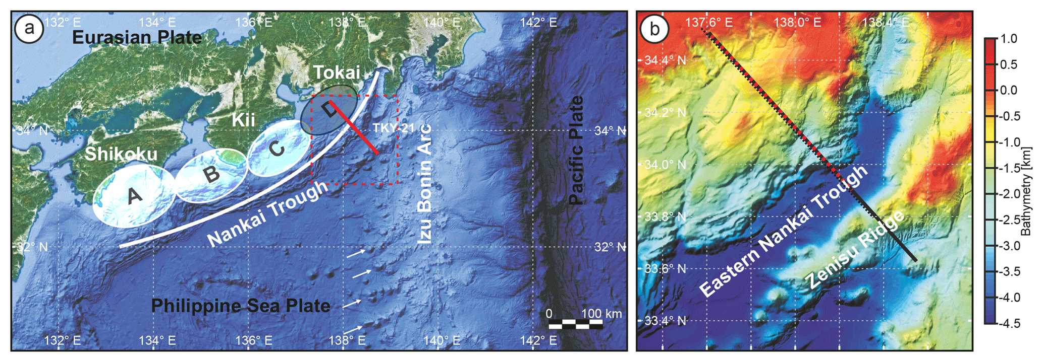
Figure 1(a) Partitioning of the Nankai Trough into four segments as described by Ando (1975). Region D was left unruptured during the most recent sequence of two large earthquakes (1944 Tonankai and 1946 Nankaido). The solid red line represents the seismic profile of the SFJ OBS experiment. White arrows mark the cyclic volcanic ridges developing on the flank of the Izu–Bonin Arc. (b) Zoomed view of the survey area, overlaid with the bathymetry variations. The solid grey line and the dashed red line represent the OBS shot and receiver profile, respectively, while the dashed black line corresponds to the MCS profile (Górszczyk et al., 2017).
The Nankai Trough, offshore of Japan, is one of the most complex subduction zone settings around the world. In this area the Philippine Sea Plate subducts below the Eurasian Plate towards the northwest, developing a large, sediment-dominated accretionary prism (Fig. 1a). The plate boundary was divided into four segments (Fig. 1a) according to the occurrence of the large earthquakes activating them every 100 to 200 years (Ando, 1975). In particular, due to the proximity of the collision zone between the Izu–Bonin Arc and central Japan, the Tokai segment (zone D in Fig. 1a) is characterized by high geodynamical complexity and the deformation of the surrounding crust. The local tectonic regime implies the formation and subduction of volcanic ridges, like the Zenisu Ridge (see Fig. 1b). Once such thickened crust enters the subduction zone, it affects the local geodynamical setting and has the potential to control the nucleation and propagation of large earthquakes (Lallemand et al., 1992; Le Pichon et al., 1996; Mazzotti et al., 2002; Kodaira et al., 2003). In the eastern Nankai Trough, the existence of such a subducted ridge (the so-called Paleo-Zenisu ridge) was first investigated by Lallemand et al. (1992) based on experimental sandbox modeling of oceanic ridge subduction and later supported by gravimetric and magnetic data analysis (Le Pichon et al., 1996). Interestingly, the Tokai segment did not rupture during the most recent large Tonankai (1944) and Nankaido (1946) earthquakes, which implies that the compressive stress has been increasing for more than 160 years. This in turn raises the question of the timing of the next megathrust earthquake (Le Pichon et al., 1996). Therefore, in order to investigate the seismogenic nature of the Nankai Trough, various data have been collected in this area. Some measurements come from passive seismic monitoring of fault zones conducted both below and on the seafloor (e.g., within the framework of NanTroSEIZE drilling program or DONET, the Dense Oceanfloor Network System for Earthquakes and Tsunamis). Simultaneously, active seismic experiments have been conducted to geophysically image and reconstruct the physical parameters of the underlying geological structure. In this study, we focus on the active seismic experiments. In particular we utilize two types of seismic data, namely MCS reflection data and OBS wide-angle data, which combined with complementary processing techniques shed new light on the deep structure of the eastern Nankai subduction zone.
2.1 Acquisition
In order to gain new insight into the crustal structure of the eastern Nankai Trough, 2-D MCS and dense OBS datasets were acquired in 2000 and 2001 as part of the Seize France Japan (SFJ) project. The profiles were roughly perpendicular to the trench axis, resulting in significant variations in bathymetry between approximately 500 and 3750 m (Fig. 1b).
During the 2001 SFJ OBS leg, the wide-angle dataset was collected by 100 OBSs spaced 1 km apart and equipped with 4.5 Hz three-component geophones and hydrophones (Dessa et al., 2004a). A total of 1404 shots were fired every 100 m along a 140 km long profile using an air-gun array with a total volume of 196 L.
A coincident towed-streamer profile was also acquired during the SFJ MCS survey (Martin et al., 2000). The total air-gun array volume (GI GUN + BOLT) was 47 L and the shot interval was 50 m. The streamer cable, which employed 360 channels distributed over 4.5 km, was towed at a depth of 15 m. These acquisition parameters result in a CMP interval of 6.25 m and fold equal to 45.
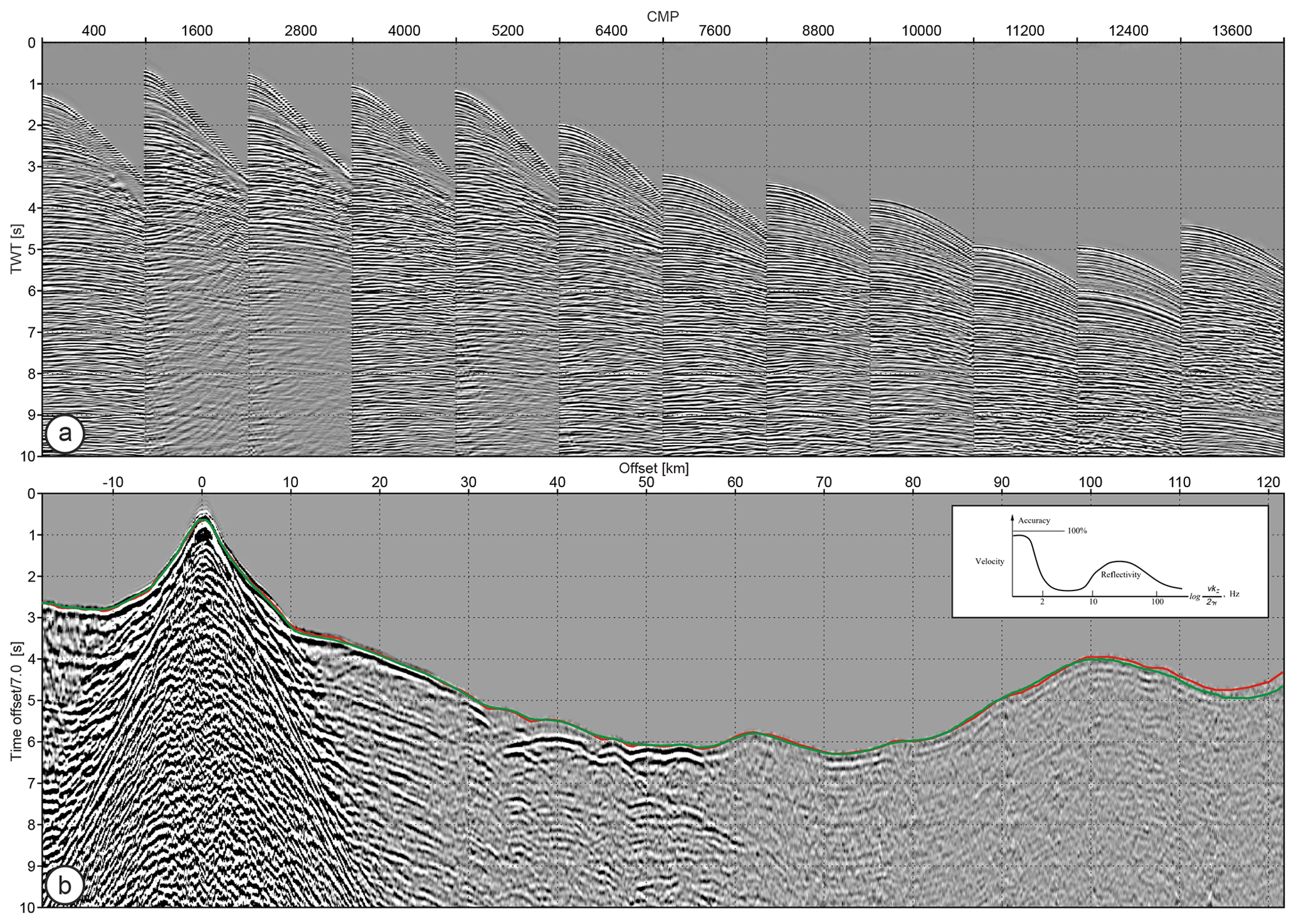
Figure 2(a) Example of MCS data sorted into CMP gathers extracted along the whole profile. Each 1200th CMP gather is displayed. (b) Example of a single OBS gather. The red and green lines show picked and synthetic travel times, with the latter being computed in the FAT velocity model. The match between the two lines gives some insight on the kinematic accuracy that may need to be achieved to prevent cycle skipping during subsequent FWI. Note also the challenging picking of first arrivals between 35 and 45 km of offset, whereby weak-amplitude first arrivals correspond to head waves that propagate along a thrust in the backstop. See Górszczyk et al. (2017) for details. Inset in (b) presents a resolution gap between tomographic velocity models and migration images (Fig. 1.13 of Claerbout, 1985)
Examples of MCS and OBS gathers are shown in Fig. 2. Both wavefields have fundamentally different anatomies and hence contain subsurface information for different resolutions and depth penetration. MCS data (Fig. 2a) typically record short-spread reflections that are sensitive to subvertical impedance contrasts, which can be imaged by migration techniques. Additionally, smooth lateral velocity variations can be updated along the two one-way transmission paths connecting the reflectors mapped by migration to the sources and receivers at the surface using either reflection travel time (Woodward et al., 2008) or waveform (Brossier et al., 2015) tomography. However, this velocity updating can be robustly performed only at relatively shallow depths at which the recorded reflection move-out is significant (∼5 km according to the 4.5 km streamer length). In contrast, OBS data (Fig. 2b) are dominated by diving waves and post-critical reflections, namely wide-aperture arrivals, which provide information on the long to intermediate subhorizontal wavelengths of the structure. Compared to towed-streamer surveys, stationary-receiver acquisitions have the necessary versatility to design long-offset regional acquisitions. At the expense of the receiver sampling they are able to record diving waves that undershoot the deepest targeted structure. For example, the first arrival shown in Fig. 2b beyond 60 km of offset is the Pn wave, namely the refracted wave in the upper mantle. Thus, integrated imaging workflows, exploiting all the information from these different wavefields, which carry different resolving power, should provide improved crustal-scale images compared with techniques employing a single methodology.
2.2 Processing
Integration of migration- and tomography-like techniques has been a common practice in seismic imaging for decades (e.g., Agudelo et al., 2009). However, when the recorded data lack low frequencies and the acquisition setup does not allow for the recording of a wide variety of wave types (transmitted versus reflected), there is a significant resolution gap between the velocity model built by tomography and the reflectivity mapped by migration (Claerbout, 1985, see inset in Fig. 2b). Recent developments of FWI technology associated with the acquisition of broadband, wide-azimuth, long-offset data aim to reduce this gap by pushing tomography and migration toward higher and lower wavenumber reconstructions, respectively (Biondi and Almomin, 2014). Although we use vintage MCS data in this study, which lack long offsets and low frequencies, the application of FWI to the OBS data (after FAT) provides an illustration of the benefit of high-resolution waveform inversion techniques applied to long-offset data, namely narrowing the resolution gap between velocity models and reflectivity.
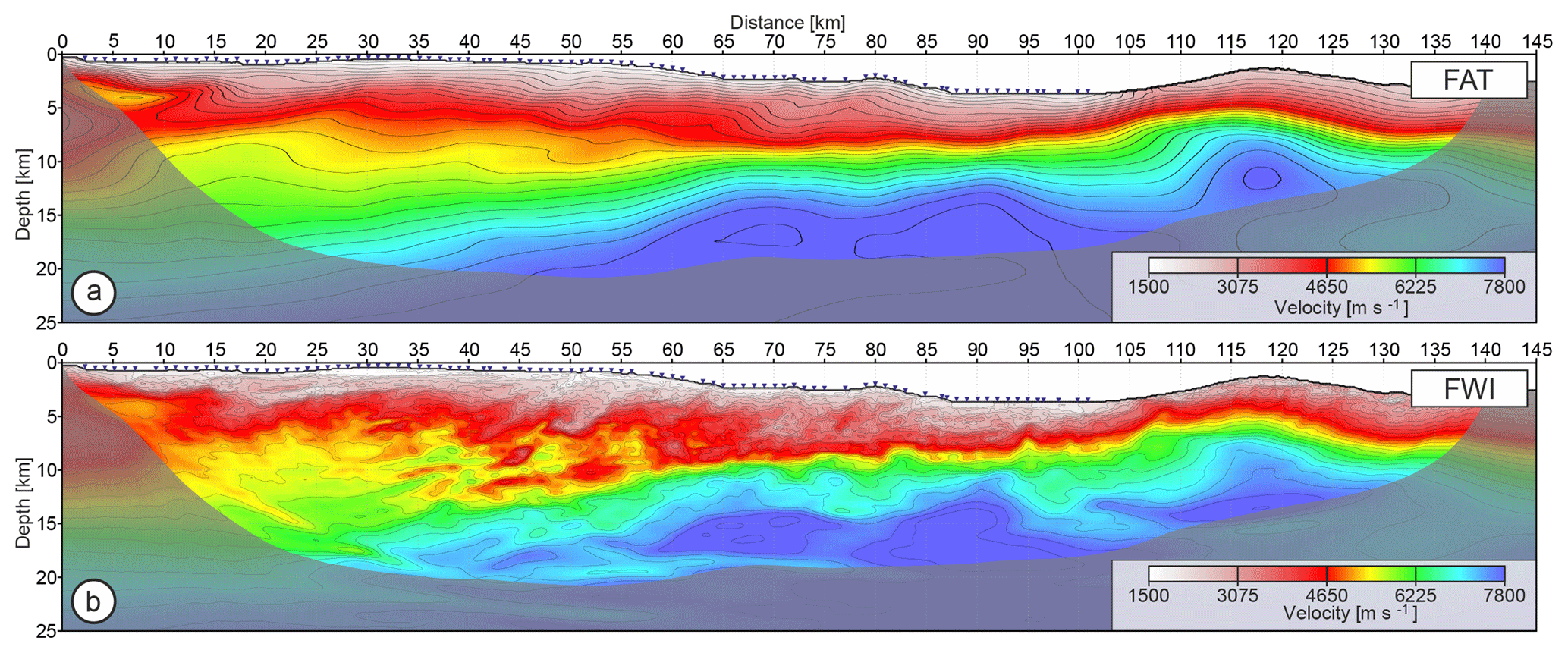
Figure 3Velocity models derived from the OBS data using FAT (a) and FWI (b). Triangles at the seafloor represent positions of the OBSs. Note that there is no OBS coverage above 102 km of distance. Shading mask corresponds to the area not covered by first-arrival rays.
To summarize the motivation behind our seismic processing workflow for deep crustal imaging, the application of FWI to OBS data have done the following: (i) led to a reliable velocity field for PSDM; (ii) provided a high-resolution velocity model reducing the wavenumber gap; (iii) significantly contributed to the geological interpretation of the imaging results; and (iv) integrated wide-angle seismic data into the depth imaging workflow of reflection seismic data.
2.2.1 OBS data
The aim of processing the SFJ OBS dataset was to obtain a crustal-scale P-wave velocity model using FWI such that it could provide insight into deep crustal targets with wavelength-scale resolution. The dataset was recently reprocessed by Górszczyk et al. (2017).
The first step consisted of building an accurate starting model using FAT. In the case of regional-scale datasets, long offsets imply that a large number of wavelengths are propagated, during which kinematic errors accumulate, hence making FWI prone to cycle skipping (Virieux and Operto, 2009, their Fig. 7). To overcome the cycle skipping issue, one needs to carefully check that the starting model predicts the picked first-arrival travel times with an error that does not exceed half of the period associated with the starting frequency (see green and red lines in Fig. 2b). In our case, we obtained a root mean square (RMS) misfit below 50 ms through iterative FAT, wherein a careful model-driven quality control (QC) of the travel time picking was performed. The resulting FAT model used as an initial model for FWI is presented in Fig. 3a.
In the next step, acoustic Laplace–Fourier FWI (Shin and Cha, 2009; Brossier et al., 2009) combined with a layer-stripping approach was applied in the 1.5–8.0 Hz frequency band. Applying strong exponential time damping of the data during the early stages of the FWI allowed us to start the inversion from a frequency as low as 1.5 Hz, which together with the kinematic accuracy of our initial model contributes to mitigating the risk of cycle skipping. A multiscale inversion approach consisted of proceeding from low- to high-frequency bands, which is combined with a continuation from wide to narrow scattering angles implemented by relaxation of the time damping of the Laplace–Fourier inversion. These two hierarchical data-driven strategies were complemented with a layer-stripping procedure implemented by progressive extension of the offset range involved in the inversion. Such a combination allowed us to mitigate the nonlinearity of the inverse problem and reduce the risk of cycle skipping accordingly.
Comparison of the final FAT and FWI models in Fig. 3 shows the significant resolution improvement achieved by FWI. Some smearing artifacts are also introduced close to the edge of the shaded area (representing the range of the first-arrival ray coverage) due to the insufficient sampling of the subsurface. Exhaustive validation, including quantitative evaluation of synthetic and real data fitting with dynamic image warping (DIW; Hale, 2013), wavelet estimation and checkerboard tests, led to the conclusion that the final FWI model reproduced the field data with high accuracy (the reader is encouraged to see Górszczyk et al., 2017, for details regarding the validation of both models).
2.2.2 MCS data – preprocessing
Processing of the SFJ MCS data was focused on the best possible reflection imaging of the subduction system. The difficulty of the task is not only due to the complexity of the underlying structure but also due to the low ratio between the streamer length and the deepest targeted structure as well as two-dimensional acquisition setting. The processing sequence is summarized in Table 1.
At the preprocessing stage, we mainly focus on the noise attenuation, wavelet corrections and multiple elimination. To improve the signal-to-noise ratio (SNR), filters designed to remove different kinds of coherent noise (e.g., swell noise, seismic interference noise, linear noise, double shots) were applied. The bubble effect was removed, followed by the zero phasing of the wavelet and reduction of the ghost on the source and receiver side.

Next, we focused on the attenuation of multiples. The lack of a general demultiple approach imposes the need to tune the processing workflow according to the limitations caused by the geological setting and the acquisition parameters. In our case, the deeply underlying complex structure causes a lot of triplications and discontinuities of the wavefield, especially at later times. Also, due to the relatively short streamer, the ability to track the move-outs is limited. This in turn confines the robustness of move-out-discrimination-based methods (e.g., utilizing Radon transform; Hampson, 1986; Kabir and Marfurt, 1999), which can easily damage the primaries if an aggressive parameterization is used. Alternatively, approaches based on multiple prediction and subtraction, like surface-related multiple elimination (SRME; Verschuur et al., 1992), could be utilized. While SRME is a data-driven technique and therefore does not require a priori knowledge about the subsurface, its assumptions can be violated in different ways by the field data. In their overview, Dragoset and Jeričević (1998) discussed in detail the limitations of SRME when 2-D data are affected by out-of-plane propagation, lack near-offset traces or contain distortions caused, for example, by the streamer feathering.
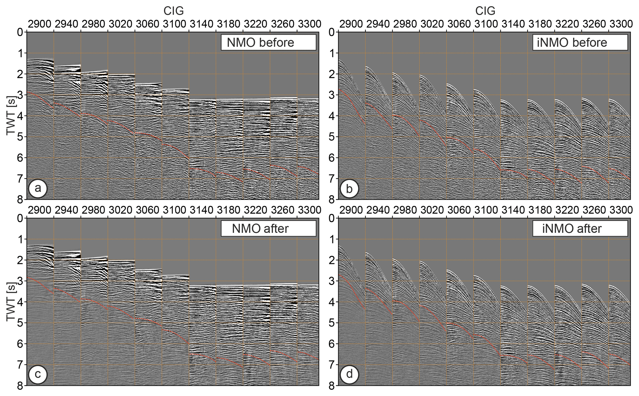
Figure 4CIGs converted to time domain (a–b) before and (c–d) after radon multiple attenuation. Gathers in (a)–(c) are NMO-corrected, while gathers in (b)–(d) have inverse NMO applied. Red dashed curves delineate the estimated position of the multiples.
In our processing scheme, we chose first to apply 2-D SRME, which is unlikely to affect the primaries. After SRME the vast majority of the free-surface multiples were attenuated. However, in certain areas of the accretionary wedge (e.g., between 55 and 80 km of the model distance in Fig. 3), we observed that residual multiples still strongly contaminated the later arrivals. These residuals are visible on the gathers presented in Fig. 4a–b both with and without normal move-out (NMO) correction applied. To further attenuate the remaining multiples we applied high-resolution radon demultiple (HRRD; Hargreaves and Cooper, 2001). Data after HRRD are presented in the corresponding panels (c–d) of Fig. 4. Note that the multiple arrivals were better suppressed now, although generally weaker signal amplitudes are observed in the processed part of the gathers. The fact that SRME was unable to fully remove these arrivals can be an indicator of out-of-plane wavefield propagation in this area associated with the complex geology and/or cross-dip inclination of the structures.
2.2.3 MCS data – velocity analysis
In this section, we will examine the issue of building a velocity model from short-streamer MCS data. In the classical VA the move-out curve is (in a typical case) approximated by the hyperbolic relationship between zero-offset time and velocity. Stacking velocities are often picked at multiple locations along a line and are further interpolated between analysis points. This procedure is usually repeated several times with the simultaneous refining of the sampling interval leading to more detailed velocity estimation (Yilmaz, 2001). The sampling of the velocity picks is supposed to be tailored by the interpreter to the degree of horizontal and vertical velocity heterogeneity defining the subsurface structure. Therefore, the ability to build an accurate velocity model via VA will firstly rely on the ability to track the move-outs, which in turn can be affected by different factors (e.g., noise, multiples, streamer length, arrival time, amplitude versus offset (AVO) variations, frequency bandwidth, velocity itself, geological structure, etc.). Secondly, it will depend on the optimal sampling of velocity picks and therefore on the initial interpretation of the data and the corresponding velocity field.
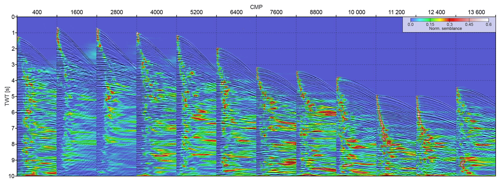
Figure 5Results of semblance-based velocity analysis performed on the gathers presented in Fig. 2a.
In Fig. 5, we present the CMP gathers from Fig. 2a extracted along the whole profile every 7.5 km. On top of them, we superimpose panels resulting from the hyperbolic semblance-based VA. Large bathymetry variations are directly reflected by the change in the magnitude of the move-outs along the profile. Thin sedimentary cover on the shallow water part of the profile (landward side) generates a smaller number of energetic reflections than the thick sediment deposits beneath the intermediate and deep water section. Move-outs are more continuous in the gathers recorded over the relatively undeformed sediments accumulated in the trench compared to the reflections originating at the steeply dipping interfaces in the accretionary wedge. Generally continuous reflections with traceable move-outs can be observed within the time window of about 2 to 3 s of two-way travel time (TWT) after the first break.
The results confirm that meaningful information from hyperbolic move-out can only be retrieved in the shallow part in which the semblance amplitudes are sufficiently well focused and allow the increasing velocity trend with time to be tracked. However, at intermediate and later times the VA panels become more chaotic and no distinct maximum semblance focusing points can be picked. This is of course a consequence of the increasing depth of the target to be imaged. Moreover, it is also worth mentioning that the final FWI model (Fig. 3b) manifests a few locations where the velocity gradient with depth becomes negative. Some of these areas are related to the existence of low-velocity zones (LVZs), which might be difficult to detect through classical VA.
2.2.4 MCS data – slope tomography
To further improve the velocity model obtained via VA, one may consider application of some variant of reflection travel time tomography utilizing information about the RMOs of reflections tracked in the CIGs after initial PSDM. Of course, the robustness of the tomographic approach relies on the precision and redundancy of the picked RMOs. In the simplest case, the velocity model is built through the minimization of the difference between travel times generated in the model with ray tracing and those measured from the data (Bishop et al., 1985; Farra and Madariaga, 1988). In addition to travel times, the slopes of locally coherent events can be picked in common-shot and common-receiver gathers and included as objective measures in the inversion (Billette and Lambaré, 1998). Development of so-called slope tomography or stereotomography proved that this technique gives a promising alternative for estimating laterally heterogeneous velocity models from reflection seismic data (see Lambaré, 2008, for a review).

Figure 6Local coherent events picked for ST. Each local coherent event is described by the source and receiver positions (s, r), the slopes (Ps, Pr) picked in (a) common-shot and (b) common-receiver gathers, and two-way travel time Tsr. (c) Data space and model space in ST. The symbols (+) denote the velocity nodes. Two rays are shot toward the source s and receiver r from the scatterer x with takeoff angles Θs and Θr corresponding to one-way travel times Ts and Tr. The velocity model, the scatterer coordinates x and the ray attributes (Θs, Θr, Ts and Tr) form the model space of classical ST. The scatterer position x and the two takeoff angles (Θs, Θr) define a dip (migration facet). The horizontal component of the slowness vectors at the source and receiver positions, Ps and Pr, the two-way travel time Tsr, and the source and receiver positions (s, r) form the data space of classical ST (adapted from Tavakoli et al., 2017).
In the data domain, the input data (picks) are defined by their source-to-receiver two-way travel time and two slopes, namely the horizontal component of the slowness vectors at the shot and receiver positions (Fig. 6a–b). For a given velocity model, each locally coherent event is associated with two ray segments (and therefore two one-way travel times) emerging at certain angles from a scattering position (whose position needs to be estimated) towards the source and receiver (Billette and Lambaré, 1998). Different variants of ST have been developed to date. Some aimed to reduce the sensitivity of the method to the quality of the input data (Biondi, 1992). Others established a connection with migration-based velocity analysis in which the picking is performed on the pre-stack-migrated volume (Chauris et al., 2002; Nguyen et al., 2008). More recently, Tavakoli et al. (2017) and Tavakoli et al. (2019) reformulated ST using the eikonal solver to perform the forward problem and the adjoint-state method to avoid the explicit building of the sensitivity matrix in the inverse problem (adjoint slope tomography – AST). This formulation leads to a more compact parameterization in which several ray attributes are removed from the model space and the shot and receiver positions from the data spaces. Following this approach, Sambolian et al. (2019) further reduced the problem parameterization to a single input data class (the slope), while inverting for the velocity parameter only. This parsimonious parameterization is achieved by using the focusing equations of Chauris et al. (2002) to position the scattering points in depth through a migration of two kinematic invariants (two-way travel time and one slope) instead of processing the coordinates of the scattering positions as optimization parameters.
One of the advantageous assumptions about the input data for ST is that the picked events need to be only locally coherent (see Fig. 6a–b). Unlike travel time tomography, it is not necessary to follow continuous arrival across the whole trace gather or follow some specified horizon (typically the interface corresponding to the specified geological boundary) (Billette and Lambaré, 1998). Tracking locally coherent events by semiautomatic picking instead of continuous reflections generally leads to denser sampling and hence a better-resolved velocity model. The attributes of locally coherent events, referred to as kinematic invariants, are simultaneously picked in the common-shot and common-receiver gathers by local slant stack (Billette et al., 2003). Alternatively, one can infer them from de-migration of the dip attribute and scattering positions picked in the pre-stack depth-migrated volume with the benefits of a better SNR and an easier interpretation or QC (Guillaume et al., 2008).
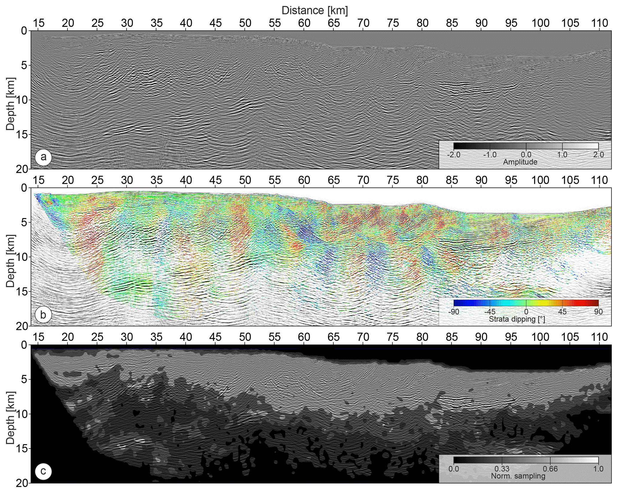
Figure 7(a) PSDM section inferred from the FWI velocity model. (b) Cloud of the scattering points corresponding to picked slopes. Colors represent estimated dipping of the interfaces. (c) Normalized average sampling of the model space by the scattering points superimposed over the PSDM section from (a).
From Fig. 7a, presenting the PSDM section computed in the FWI model, one can easily spot the areas of stronger and weaker reflectivity. To further update the FWI model via ST one needs to track locally coherent events, and therefore the areas of lower reflectivity might be poorly constrained by the picked data. To gain insight into which part of the model space was well constrained by our ST picks, in Fig. 7b we show the PSDM section from Fig. 7a overlaid with the cloud of scattering points positioned through the migration of the kinematic invariants. The color palette corresponds to the dip of the migrated facets. These dips are defined by the sum of the takeoff angles of the two rays emerging at the scattering position and ending at the shot and receiver positions. Color variations highlight the consistency of the picked scattering points with the underlying geology. The cold-colored dots (blue, light blue and cyan) follow seaward-dipping structures, while warm-colored dots (yellow, orange and red) trail the interfaces of opposite inclination. Not surprisingly, the number of picks decreases significantly with increasing depth, although we can observe quite a dense set of picks around the plate interface on the landward side between the backstop and subducting oceanic plate at a depth of around 15 km. The fact that the corresponding events were picked at this depth confirms the high accuracy of the FWI model; however, in the case of short-streamer data the sensitivity of move-outs to velocity changes at this depth is rather low.
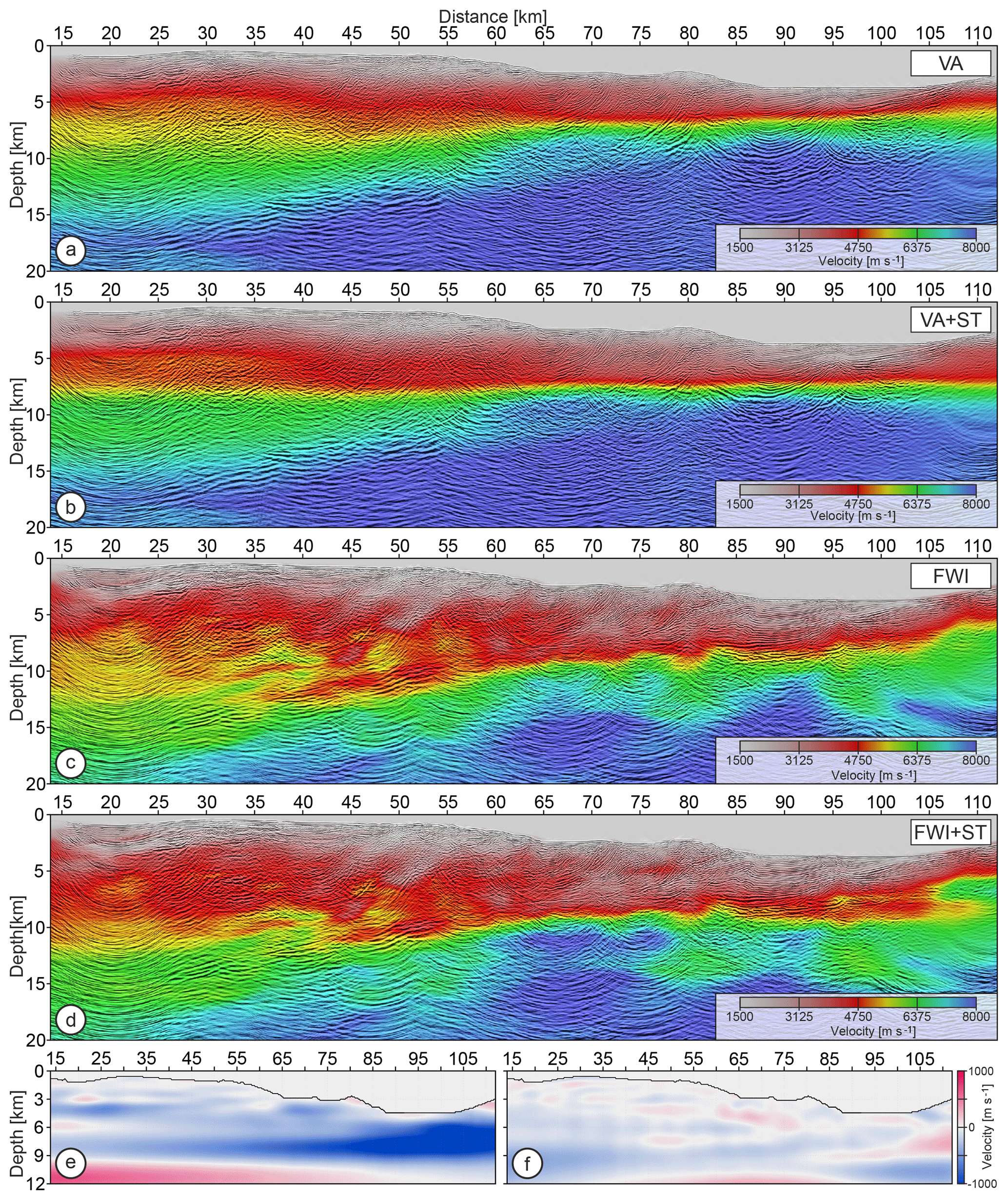
Figure 8PSDM sections inferred from the (a) VA, (b) VA+ST, (c) FWI and (d) FWI+ST velocity models displayed in the background. Velocity perturbations introduced by ST into the (e) VA and (f) FWI velocity models.
It is worth mentioning here that in Fig. 7b between 60 and 85 km of model distance and below 10 km of depth we observe a collection of scattering points with variable conflicting dipping (interleaved color-scale changes: cold–warm–cold–warm–cold–warm). This cloud of picks matches the strong events that have not been migrated properly with any available velocity model (including velocity scaling) and appear in the PSDM section in the form of so-called migration smiles. The corresponding area of the FWI model after ST update (Fig. 8d) exhibits locally unrealistic velocity values in the upper oceanic crust (∼8000 m s−1). Although generally higher velocity values are observed in this area both in the FAT and FWI models, the evidence of migration artifacts combined with some overestimated velocities after ST might suggest the out-of-plane propagation of the wavefield in this complex geological setting.
To express in a more quantitative way the relative sampling of the model by the picks we calculate their hit rate inside square grid cells of size 0.5 km. Consequently, we clip 10 % of the highest values, normalize the results between 0 and 1, and divide them into three uniform intervals. Figure 7c presents the PSDM section with superimposed shading masks corresponding to the normalized sampling of the model by picks. The brightest area of the section was sampled between 100 % and 66 % of the maximum (clipped) pick hit-rate value. The next two grey-shaded areas were sampled between 66 % and 33 % and between 33 % and 0 %, respectively. The black area defines the part of the model not sampled by picks.
To conclude we can make the statement that the robustness of the ST method is reflected by the distribution of the scattering points demonstrating high consistency with the dipping structures observed in the PSDM section. This in turn ensures regular and redundant information that might be exploited for velocity model building. However, the number of picks and their robustness (especially during 2-D processing) are significantly reduced with depth as the reflectivity of the structure decreases. This is more pronounced on the landward part (backstop) of the model. Therefore, the constraints on the velocity model at larger depths, although significantly better than those provided by classical VA, are weaker than in the shallow section.
2.2.5 PSDM
During the PSDM step, we tested different background velocity models, targeting the optimal flattening of the CIGs. Here we consider only four of them. The first one was built from MCS data by classical VA, while the second one is the FWI model inferred from the OBS data (Fig. 3b). In this sense, PSDM of MCS data can be seen as an additional QC on the FWI model. We expect both the VA and FWI models not to be strictly precise for PSDM of MCS data at such a geological scale (in the first case because of the lateral-homogeneity assumption of classical time-domain VA; in the second case because the wide-angle seismic data are used to build the velocity model for reflection data). To further check how much we can improve the PSDM results by refining these velocity models, we perform RMO picking in the pre-stack-migrated gathers that were subsequently minimized by ST. Therefore, through the ST we also assess the accuracy of both velocity models for PSDM (small modifications of the model indicate its robustness) and optimize the imaging result. The original and refined velocity models produced four PSDM images. We essentially tested Kirchhoff PSDM as well as controlled beam migration (CBM) with the aim of improving the SNR of the final result (considering our low-fold dataset). CBM is an extension of beam migration technology, which combines the steep-dip imaging capabilities of Kirchhoff techniques with the multi-arrival abilities of wave-equation migration (WEM) (Vinje et al., 2008). The results obtained with both migration techniques, however, did not provide a clear indication of which approach was superior, and therefore, for simplicity, we decided to adopt PSDM in the classical Kirchhoff version.
In the following sections we present the PSDM results inferred from the four abovementioned background velocity models. We assess them by looking at the flatness of the CIGs as well as through the correlation of the migrated sections with the underlying velocity models. Furthermore, we compare the main observed structures against the results reported by previous geological studies conducted in this area.
3.1 Imaging
The PSDM sections, superimposed on the VA- and FWI-related velocity models with which they were computed, are presented in Fig. 8. Amplitudes of the stacks were scaled with a power function of depth (power equal to 1.5). Generally, all PSDM sections exhibit similar quality in the shallow seabed area (first 2–3 km). However, the PSDM sections obtained with the FWI and FWI+ST velocity models (Fig. 8c–d) show better-focused reflectivity at intermediate and large depths. This is especially pronounced below the accretionary prism (5–10 km of depth, 55–100 km of distance) as well as in the landward-dipping subducting oceanic crust down to about 15 km of depth.
We validate resulting PSDM sections against the corresponding background velocity models. The structure imaged in PSDM sections inferred from VA velocity models is less well focused than in those inferred using the FWI models. This is a consequence of the fact that VA models lack resolution and accuracy due to the estimation method. Comparing panels (a) and (b) in Fig. 8, one can observe that the VA-related velocity models exhibit a similar level of smoothness, although the PSDM section corresponding to the VA model updated by ST (Fig. 8b) looks more geologically relevant. The main changes in the PSDM sections computed with the VA and VA+ST velocity model are shown in the area where ST introduced the most significant velocity updates. These perturbations are shown in Fig. 8e. The color scale was clipped at ±1000 m s−1 for better readability; however, the lowest-velocity perturbations (dark blue) reach −1500 m s−1, providing some indication of the inaccuracy of the VA model.
Analogous comparison of the FWI and FWI+ST velocity models and related PSDM sections (Fig. 8c–d) leads to the following conclusions. First, the high-resolution FWI model provides a more focused PSDM image (Fig. 8c). Second, the reflectivity image nicely follows the absolute velocity changes mapped by the FWI model. Third, the updated FWI+ST model marginally improves the final PSDM section (Fig. 8d). This improvement results from relatively small velocity perturbations introduced in the FWI model by ST (compare Fig. 8e–f). Also, the ST damages some dipping velocity structures that are more visible in the FWI model than in the FWI+ST model (see backstop between 5 and 10 km of depth or accretionary prism between 65 and 85 km of distance). The last effect is related to the nature of the perturbations typically introduced by reflection data that are more sensitive to the vertical velocity variations. In contrast, the long-offset OBS data are better suited to capture the horizontal and steeply dipping velocity changes.
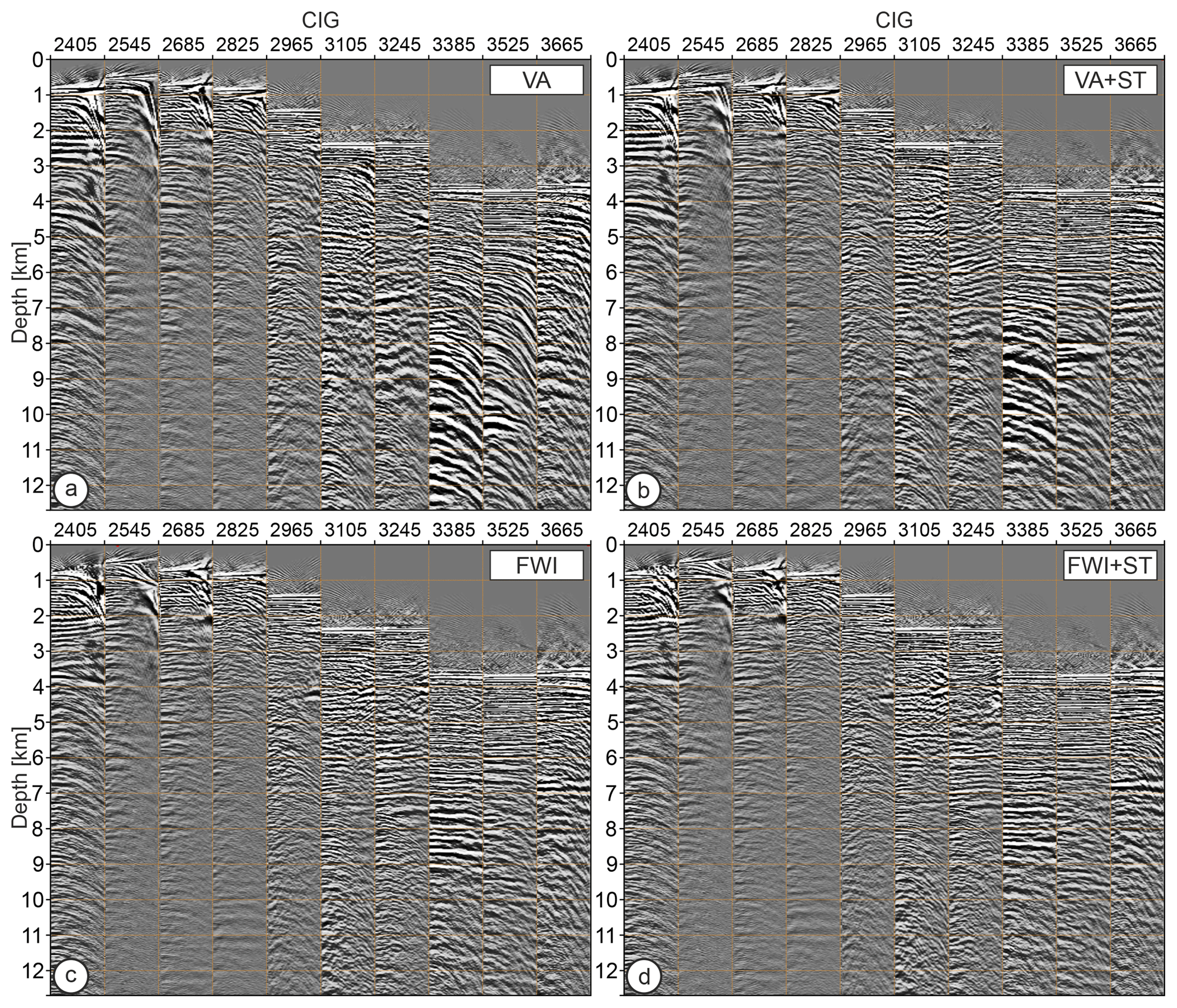
Figure 9CIGs extracted along the whole profile (every 8.75 km). (a–b) CIGs inferred from the velocity model built by (a) VA and (b) VA+ST. (c–d) CIGs inferred from the (c) FWI and (d) FWI+ST velocity models.
To further QC the imaging results in Fig. 9 we present a set of CIGs after PSDM using each of the four velocity models. The CIGs inferred from the VA model (Fig. 9a) show that only shallow events were flattened, while the intermediate and deeper reflections have strong under-corrected RMOs, indicating that the velocities are too fast. After updating the VA model using ST and running PSDM, the events are flatter (Fig. 9b). However, under-corrected RMOs are still visible in the deeper part of the gathers. Additionally, we start seeing some overcorrected reflections (e.g., CIG 3245), indicating velocities that are too slow. For comparison, CIGs inferred from the final FWI model (Fig. 9c) show that the majority of reflections are flat, including those originating from the deep crust. Refining the FWI model by ST (Fig. 9d) introduces rather local and moderate improvements in terms of the flattening and position of the reflections.
The overall trend after ST is the upshifting of the reflectors, suggesting that the velocity refinement by ST mainly lowers the FWI velocities. This likely highlights the imprint of the anisotropy. The velocities estimated by FWI are close to the horizontal velocities, while those constrained by MCS data are closer to the velocities associated with normal move-out. In all cases, RMOs are more pronounced at the side edges of the profile. The effect is caused by the lack of coverage in these areas, which translates to weak constraint during velocity model building.
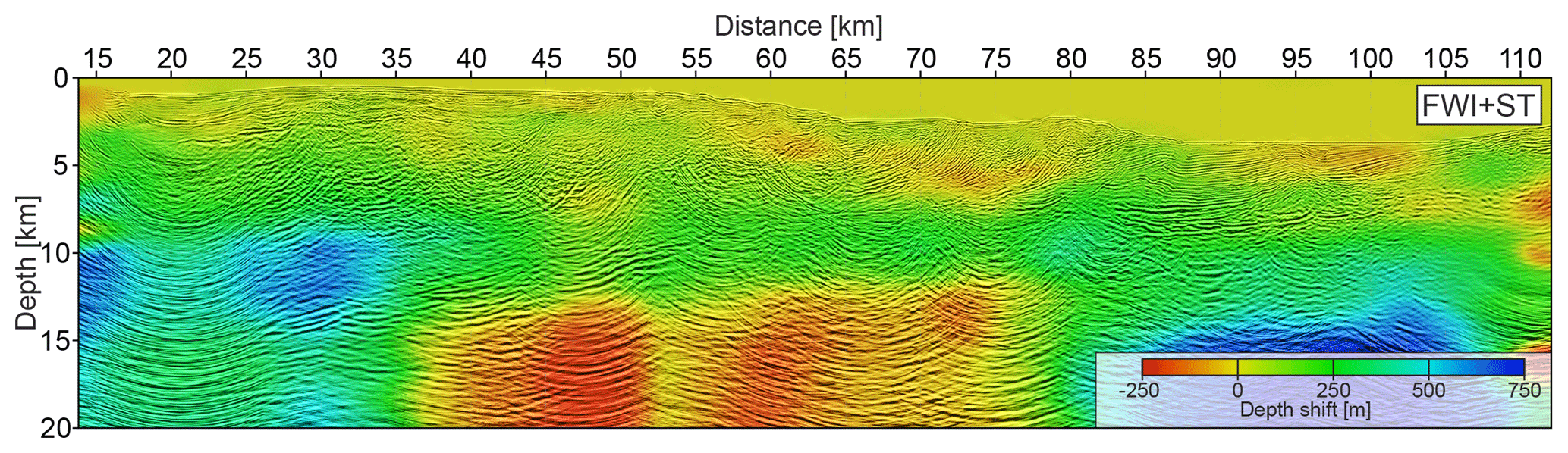
Figure 10PSDM section inferred from the FWI+ST velocity model overlaid on the estimated depth shifts. Positive and negative values correspond to upshifts and downshifts introduced in the PSDM section by FWI+ST velocities relative to the FWI velocities, respectively. Note the nonsymmetric color scale.
To quantitatively express the depth changes in the PSDM results introduced by the ST update of the FWI model, we estimate the depth shifts between the PSDM sections inferred from FWI and FWI+ST models. We calculated the local cross-correlation for each pair of corresponding traces from the mentioned sections, which led to consistent map of depth changes between them. Figure 10 shows the PSDM section inferred from the FWI+ST velocity model with an overlaid color map corresponding to depth shifts varying from −250 to 750 m. The most significant differences are observed at the left and right flanks of the section. In these areas, after ST, we observe upshift of the interfaces of about 500 m near the landward plate boundary of the subducting oceanic crust and about 750 m around Moho below the trench. In the central part of the migrated section, shifts are relatively smaller, of the order of 100–200 and 0–50 m in the oceanic crust and the accretionary prism, respectively. Such a distribution of the depth shifts results most likely from the fact that the central part of the FWI model is well sampled from both sides by the various diving waves and wide-angle reflections. In contrast, deeper parts located at the edges of the model are mainly illuminated by Pn waves propagating mainly horizontally and sporadic PmP reflections. This confers more degrees of freedom to ST for introducing changes in the velocity model, although there is limited sensitivity of the short-spread reflection data to velocities at these depths, and the possibility to pick some migration artifacts.
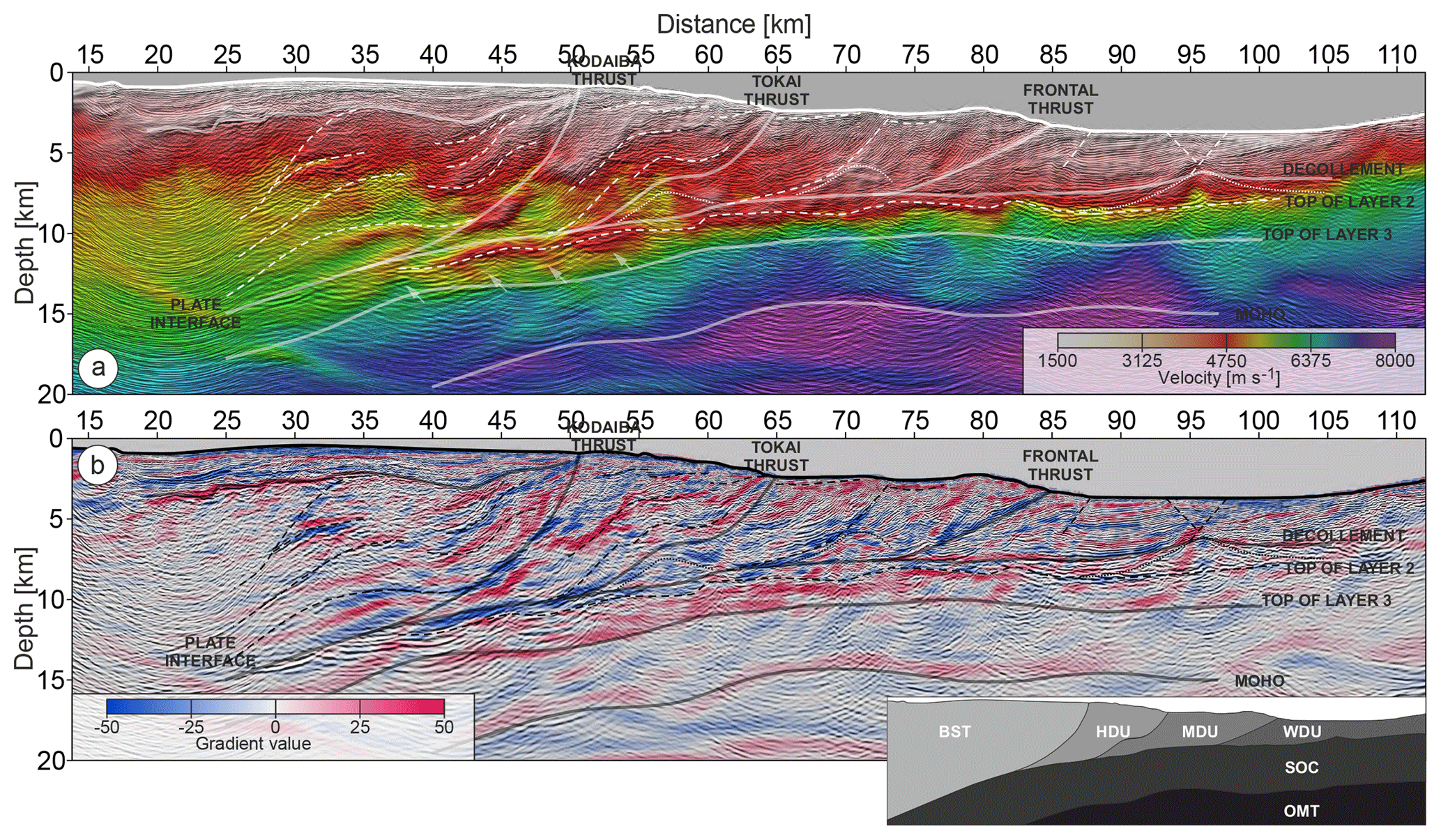
Figure 11Imaging results and structural interpretation. Migrated section superimposed on the following: (a) the FWI velocity model blended with the average vertical and horizontal velocity gradient; and (b) the average vertical and horizontal velocity gradient of the FWI model. Inset presents different geological block segments: OMT – oceanic mantle; SOC – subducting oceanic crust; WDU – weakly deformed unit; MDU – moderately deformed unit; HDU – heavily deformed unit; BST – backstop.
3.2 Geological consistency
Before interpretation, we filter out (using curvelet transform; Górszczyk et al., 2015) some of the strong migration smiles apparent in the final PSDM sections, which after analysis in the pre-stack domain have been addressed as residual multiples or out-of-plane arrivals. To foster the joint interpretation of the PSDM results and FWI velocity models, we overlay the migrated section on the (i) FWI model, (ii) velocity gradient image, i.e., the average of the horizontal and vertical derivative of the FWI velocity model (Fig. 11a–b), and (iii) perturbation model – the FWI model after removing the velocity trend obtained by fifth-order polynomial fitting each vertical profile of the FWI model (Fig. 12a–b). The resulting sections provide not only an image of the reflectivity but also a high-resolution background insight into the seismic properties (P-wave velocity changes) of the structural units delineated by the reflectors. The resulting images show the high consistency between the velocity structures and the reflectivity image, improving the continuity and delineation of some interfaces that are locally more visible in the PSDM section than in the velocity model and vice versa. Based on the deformation features and the velocity structures identified in the obtained images, we classify the geology of this region into block segments including different deformation domains (see inset in Fig. 11b), which are bounded by three major faults and the basement, namely the subducting plate interface.
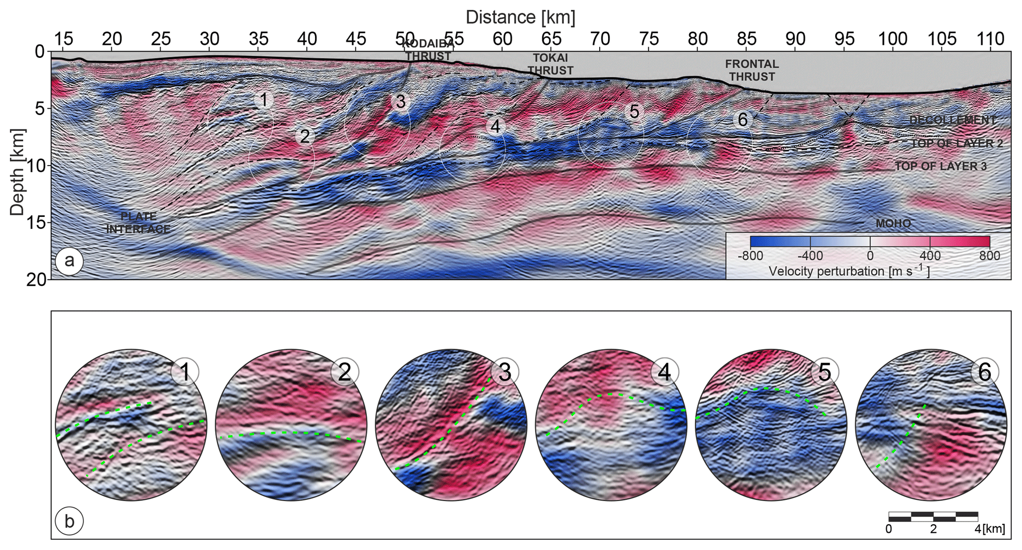
Figure 12Imaging results and structural interpretation. (a) Migrated section superimposed on a de-trended version of the FWI velocity model, blended with the average vertical and horizontal velocity gradient. (b) Zoom panels corresponding to circles 1–6 in Fig. 12a. Green dashed lines underline the consistency between reflectivity and background velocity perturbations.
3.2.1 Structure of the subducting oceanic crust
The oceanic crust in the region of Tokai is commonly described as being affected by volcanism (Le Pichon et al., 1996; Nakanishi et al., 1998; Martin, 2003; Mazzotti et al., 2002; Dessa et al., 2004b; Kodaira et al., 2002; Takahashi et al., 2002). The main reason for this is the proximity of the Izu–Bonin Arc, which develops periodical volcanic ridges on its western flank (see white arrows in Fig. 1a) that are further subducted beneath central Japan. Moreover, the geodynamic setting of this region is further under the influence of the Izu Arc colliding with central Japan as well as the initial thrusting stage around the Zenisu Ridge. Such a setting can explain the deformed shape of the subducting oceanic crust with the local increasing and/or lowering of velocity values observed in Fig. 11a as well as weak and rather difficult to distinguish reflectivity within the subducting crust. In the resulting images, the Moho boundary is derived from both the absolute velocity model (Fig. 11a) and the positive change in the gradient value (red) in Fig. 11b. The migrated image at this depth (not surprisingly, owing to the 4.5 km streamer length) is strongly affected by migration smiles. To support the interpretation of upper mantle one can additionally calculate refraction ray tracing in the final FWI model and track the rays corresponding to Pn arrival, which tend to propagate just below the Moho boundary (see Fig. 13e in Górszczyk et al., 2017, for the illustration).
In Fig. 11b in the upper part of the oceanic crust one can identify a ∼3 km thick band of positive gradient (red) interpreted as layer 2. This significant gradient vanishes around the solid line corresponding to the top of layer 3. The top of layer 2 is marked with the dashed line following a discontinuous reflectivity package between the décollement and the top of layer 3. In both Figs. 11a–b and 12a we observe step-like velocity variations around this dashed line at model distance 82, 73, 59 or 53 km. The velocity changes correlate with discontinuities of reflections (see, e.g., Fig. 12b zoom panel 6), which further extend with depth into migration artifacts. This observation is consistent with the proposed system of major faults offsetting various reflectors across the whole oceanic crust in the region of the Nankai Trough (Dessa et al., 2004b; Kodaira et al., 2002; Tsuji et al., 2013; Lallemand, 2014). Some of these faults can act as a paths for fluid migration, causing alternation of the deep rocks (e.g., serpentinization), which may be a further reason for rapid velocity variations within the subducting oceanic crust. Such fluid–rock interaction and velocity alteration have also been reported at the outer ridge of the Tohoku margin (Korenaga, 2017). Above the top of layer 2 with a solid line we interpret the top of the sedimentary subduction channel acting as a décollement, which is relatively well supported by reflectivity on the PSDM image and by the high-resolution velocity gradient changes.
Between 40 and 55 km of model distance we clearly identify the negative velocity gradient creating a major LVZ. The top of this LVZ is consistent with the plate interface. In our case, access to the high-resolution velocity model directly indicates a negative velocity gradient, which could alternatively be obtained from the polarization reversal in the reflectivity image addressing, for example, the presence of fluids. However, at this depth we observe several ringing reflections (see arrows in Fig. 11a) rather than a clear interface, suggesting a relatively thick layer of accumulated deformed material. Discontinuous reflection patterns can be explained by the clastic deposition or duplexing of sedimentary or volcanic material (Gutscher et al., 1998b, a). Alternatively, the LVZ can be interpreted as a damage zone caused by a topographic high passing through this area. Regions of similar nature were identified by Bangs et al. (2009) in the western part of the Nankai Trough. The plate interface can be further tracked as a landward-dipping interface reaching about 15 km of depth at 25 km of model distance. Generally higher velocity and large-scale perturbations visible in the gradient model above the plate interface in this area (25–40 km of distance) indicate the significant underplating of the subducting material and its incorporation into the backstop, simultaneously causing uplift of this part of the prism clearly visible in the shallower section.
3.2.2 Subduction front and recent accretionary wedge
On top of the subducting oceanic crust, our seismic imaging results reveal the complex accretion system of the Tokai segment, which can be divided into four domains. The weakly deformed domain is located at the southeast of the profile starting at ∼85 km of model distance (although some smaller deformations pop up around 87 km) and bounded by the western flank of the Zenisu Ridge. This domain is composed of clastic turbidite sediments deposited on the volcanic basement, creating the continuous reflection surfaces visible in the gradient model and PSDM image. One can easily observe a cone-like structure (dotted line) at 95 km with two faults originating at its apex. It most likely corresponds to a subducting volcano considering the decay of velocity within the oceanic crust below it (Fig. 11a) The subhorizontal solid line between 80 and 95 km of distance marks the strong reflector identified as an extension of the décollement since the deformation of the sediments accumulated in the trench starts to occur above this interface.
The weakly deformed domain is separated form the accretion front – a moderately deformed domain – by the major frontal thrust fault, which generates ocean-floor topography at 85 km and reaches the décollement around 13 km further in the landward direction (Hayman et al., 2011). The whole domain shows similar reflection patterns to the weakly deformed domain, suggesting that it consists of sedimentary layers, but they are folded and offset by several thrust faults reaching the detachment interface. The consistency of these thrusts with the velocity models is striking even in the small details. For example, gradient variations in Fig. 11b consistently follow the steeply dipping stacked sheets of sediments in the accretionary prism. In Fig. 12a, shallow-slope basins are clearly delineated in blue and separated by the thrust, creating a bathymetric outcrop at 73 km. Similar consistency can be observed in terms of the vanishing reflectivity of the PSDM image above the décollement between 67 and 75 km (dotted line, zoom panel 5), which is nicely delineated by lower velocity values indicated by blue. Interestingly, the décollement on the right side of this feature manifests itself in Fig. 11b as a positive (red) gradient, while on the left side it becomes opposite (blue), suggesting a decrease in velocity.
3.2.3 Tokai thrust and subducting Paleo-Zenisu ridge
The moderately deformed domain extends landward until the Tokai thrust, separating the frontal part of the prism from a heavily deformed domain (Kawamura et al., 2009; Hayman et al., 2011). This segment in turn shows less pronounced reflectivity, but the interpretation can be significantly augmented using the pattern of velocity changes in the absolute, gradient and de-trended velocity models. The structural characteristics of this domain are different from the two previous deformation domains, suggesting that it has undergone a longer period of deformation at this margin (according to Martin et al., 2003, starting at the Upper Miocene). In particular, the significant increase in the velocity values just above the plate interface (Fig. 11a), combined with a lack of clear impedance contrasts and uplifted bathymetry, suggests old accumulated material atop the plate interface. Alternatively, the increase in the velocity and strong deformation within this wedge between 50 and 65 km (dashed line) may indicate a topographic high (namely, evidence of the Paleo-Zenisu ridge) whose left flank is colliding with the old accreted thrusts (dotted line between 55 and 60 km of distance). We can also observe in Fig. 12a–b (zoom panel 4) that the small topographic pop-up is separating two areas of blue, indicating zones of lower velocities. Such a geometry suggests that the Tokai thrust is rooted at the down-stepping plate interface, follows up the left flank of this velocity anomaly, then bends above it and increases the dip again to reach its outcrop at the seabed.
We also observe that the thickness of slope sediments in the shallow part of this segment (50–63 km; blue in Fig. 12a) is larger than in the case of shallow sediment basins on top of the moderately deformed domain. This suggests a longer time of accumulation and partial erosion of the uplifted, steeply dipping thrust sheets around the Kodaiba Fault, a major thrust fault with significant strike-slip displacement (Pichon et al., 1994). Strong gradient variations in Fig. 11b delineate the geometry of this fault, especially above the plate interface. High consistency of the PSDM image and velocity changes can also be observed in Fig. 12a–b (zoom panel 3). We root this fault at the plate boundary, suggesting splay-fault branching. Alternatively, it can originate at the deep backstop on top of underplated material that might be suggested by zoom panel 2 in Fig. 12. More detailed geological investigation is necessary to confirm speculations about this fault that potentially governs the seismogenic setting in the Tokai segment.
3.2.4 Backstop area
Finally, on the most landward part of the profile, we image the old deformation complex that now acts as a backstop. The deformation of large landward-dipping stacked thrust sheets can be identified by velocity changes correlating with reflectivity visible in the PSDM image. No active deformation can be clearly identified in this area (in contrast to the frontal area of the prism see Yamada et al., 2014). The recent seismic imaging results (Shiraishi et al., 2019) derived from the 3-D MCS data recorded in the more central part of the Nankai area (the Kumano fore-arc basin) reveal a similar example and the underlying old accretionary prism that is not actively deforming. In the Tokai area, the hypothesis that this old complex could have been pushed landward by large subducting ridges was based on the results of wide-angle seismic experiments (Kodaira, 2000; Nakanishi et al., 2002) as well as sandbox tests (Dominguez et al., 2000). Placing our results in this context would require further geological expertise. Nevertheless, from the joint interpretation of velocity models and the PSDM section one can divide this domain into (i) the thick relatively undeformed sediment cover of the fore-arc basin, suggesting that the (ii) underlying complex of large thrust sheets between 4 and 10 km of depth is inactive and overlies the (iii) significant amount of underplated material delineated by the increase in velocity at a depth of around 11 km.
4.1 MCS data penetration at depth
The ability of the seismic wavefield to penetrate the deep crust is limited by various factors, including acquisition geometry, employed equipment and geological context. Sufficiently dense shot coverage increases the fold and therefore spatial sampling redundancy. The ability to generate and record broadband frequency signals improves resolution and the signal-to-noise ratio. Long streamers, although challenging to operate in the field, provide large enough offsets to track the move-outs of later arrivals originating from deep interfaces. All these factors improve the ability of MCS data to retrieve meaningful information about the deep crust. Our MCS data were recorded using a 4.5 km long streamer, which is quite limited compared to industrial 15 km long streamers. Nevertheless, we have shown that the robust depth imaging of legacy data with short offset and limited fold is possible when supported by velocity model building based on FWI of wide-angle stationary-receiver data. Despite the different regimes of wavefield propagation between wide-angle and reflection data, our FWI model provided an accurate velocity field for PSDM. This accuracy allowed for the picking of slopes for ST and introduced relatively small velocity changes even at greater depths (∼15 km). In contrast, the velocity model obtained via VA was too inaccurate to allow for similar PSDM accuracy after ST update. Therefore, building a high-resolution FWI velocity model from wide-angle OBS data can significantly improve the PSDM results from short-streamer MCS data, especially in terms of velocity accuracy below a shallow sub-seabed.
4.2 2-D and 3-D PSDM
Two-dimensional seismic data processing is inherently inaccurate because of the three-dimensional wavefield propagation within the lithosphere, which takes place during field experiments. Therefore, the assumption of inline scattering along the shooting profile is unrealistic. Nevertheless, despite the improved accuracy of a 3-D experiment, 2-D surveys remain a practical approach to retrieving geological information about the subsurface. This in turn capitalizes on limited prospects for subsequent processing (for example, the accuracy of retrieved seismic attributes) and the following quality of the results when cross-dipping structures are expected in the vicinity of the 2-D profile. While the imaging of deep crustal targets requires a long time for wavefield propagation, it means that the wavefront is also more prone to travel out of the 2-D profile plane. The complexity of the geological structures that we aimed to reconstruct here combined with their significant depth lead us to believe that the final imaging results are affected by “3-D effects”, reducing the continuity of the deeper interfaces. This was also apparent from the locally occurring arrivals that were stacking into migration artifacts. We decided to filter them out before final interpretation as we were unable to flatten them with any velocity model, even with velocity scaling ranging between 80 % and 120 %. To overcome such issues, one can consider cross-dip processing that takes into account the 3-D character of the data (for example, feathering of the streamer) and the geology (Nedimović et al., 2003). However, ultimately we believe that there is a need to move toward future 3-D experiments tackling the problem of complex deep crustal imaging (Morgan et al., 2016). Indeed, the illumination of the structure from different azimuths would increase the reliability of the final image and minimize the amount of speculation in the geological interpretation. On the other hand, this development needs to be combined with the efficient acquisition logistic schemes and robust processing techniques able to handle large-scale imaging problems.
4.3 On subducted oceanic ridges
The typical problem from the Tokai region, which can justify the use of 3-D rather than 2-D crustal-scale imaging, is the existence of the basement volcanic ridges and mountains subducting below the accretionary wedge and affecting the geodynamical setting of the region. While their existence is undeniable (even from the bathymetric observations in Fig. 1a), the exact shape and scale of those features in historical studies utilizing reflection or wide-angle seismic imaging and velocity model building, sandbox experiments, or gravity and magnetic anomaly analysis are rather inconsistent. Moreover, representing these ridges as continuous features of uniform height is oversimplified. To better understand the problem it is enough to look at how in Fig. 1b the Zenisu Ridge rapidly changes its height along the axis with respect to the trench from nearly 3 km to a few hundred meters. Therefore, to precisely image and investigate the influence of such chains of distributed volcanoes of various size subducted below the complex accretionary prism, 3-D imaging is required.
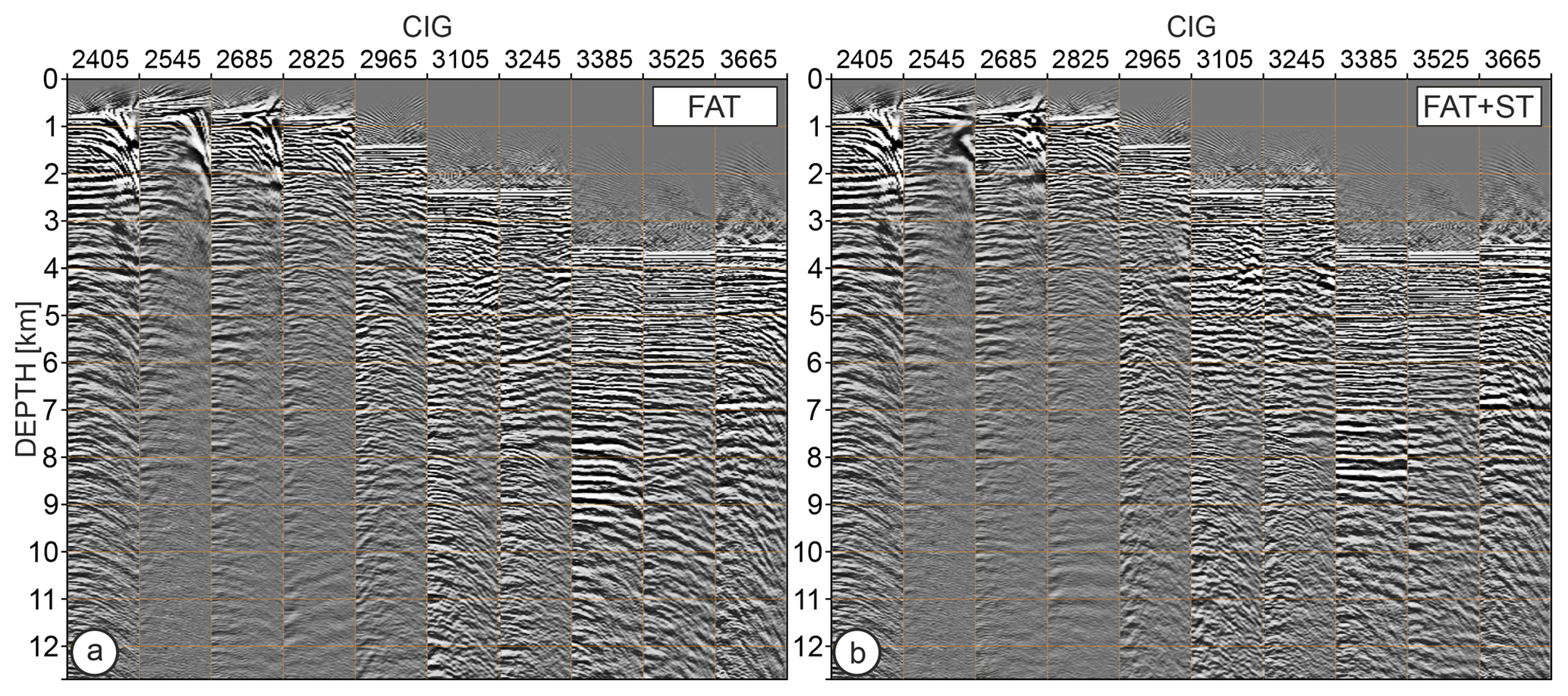
4.4 PSDM using FAT model
FWI in its classic form is a local optimization problem. In other words, the misfit functional representing the difference between real and synthetic data is iteratively minimized (towards a global minimum), starting from the initial model that is sufficiently close to the true one, such that it fulfills the cycle skipping criterion. If this condition is not met, FWI will be guided towards a local minimum and an inaccurate model. Therefore, the accuracy of the initial FWI model determines the correctness of the final results. In this sense, the robustness of the initial FWI model (in our case derived by FAT) can also be verified through PSDM. Indeed, if the velocity values in the FWI model are searched for in the vicinity of the FAT model, then PSDM utilizing the FAT model should also provide good results. To investigate this issue we performed two additional PSDM tests considering the FAT model and its version updated by ST. Figure 13 presents an analogous comparison of PSDM gathers as in the case of Fig. 9. After careful inspection of the migrated events we can conclude that the flatness of the CIGs inferred from the FAT model is locally worse than those inferred from the FWI model in Fig. 9c. Overall, however, these results are much better than those obtained with the VA and VA+ST velocity models (Fig. 9a–b). This shows how wide-angle data can be useful to build correct velocity models for PSDM using the classical FAT technique. In our case, this approach outperforms the results of PSDM with the classical VA model as well as its updated version with a rather sophisticated ST method. On the other hand, one can argue that the improvement of PSDM results obtained with FWI compared to FAT is not proportional to the efforts devoted to applying FWI. Note, however, that the smooth FAT model is unable to bring detailed structural information that is directly accessible from the high-resolution FWI model, and therefore we believe that moving from FAT to FWI is absolutely crucial for better geological interpretation.
The presented case study shows that crustal-scale FWI of OBS data can significantly improve depth-migrated images inferred from towed-streamer data. Firstly, the final FWI model provides reliable information about the velocity not only at shallow depths (<5 km) but also at depths down to the upper mantle, which are beyond the range of typical streamer length. These more reliable velocities translate to better-focused PSDM at depth. Secondly, a high-resolution FWI velocity model brings quantitative information on the seismic properties of the main structural units at long to intermediate scales, which are complementary to the short scales mapped in the PSDM image. This justifies the use of crustal-scale FWI models derived from wide-angle data for geological interpretation. We believe that further development of crustal-scale imaging toward 3-D OBS acquisition and 3-D multiparameter viscoelastic FWI will bring us closer to better understanding deep crustal targets through joint wide-angle and reflection data processing.
The data used in this research are not publicly available. The OBS and MCS data were provided based on the collaboration between Institute of Geophysics, Polish Academy of Sciences and participants of SFJ project.
AG initialized and led the research at all stages, derived FAT and FWI models from the OBS data, performed PSDM of the MCS data, conducted majority of the quality control of the results, derived initial geological interpretation, generated the figures, wrote the initial manuscript and coordinated its revision. SO co-supervised the project and participated in the design of the processing workflow and quality control of the results as well as reviewing the manuscript. LS performed the preliminary processing of SFJ-MCS data and provided the initial velocity model derived form the classical velocity analysis. YY participated in the geological interpretation of the results and participated in writing and reviewing the corresponding part of the manuscript.
The authors declare that they have no conflict of interest.
This article is part of the special issue “Advances in seismic imaging across the scales”. It is not associated with a conference.
This study was partially funded by the SEISCOPE Consortium (https://seiscope2.osug.fr, last access: 27 May 2019). This study was granted access to the HPC resources of (a) CYFRONET (https://kdm.cyfronet.pl, last access: 27 May 2019; grant ID: 3dwind), (b) CINES/IDRIS (allocation A0050410596 made by GENCI) and (c) SIGAMM (https://crimson.oca.eu, last access: 27 May 2019). The authors thank Romain Brossier and Ludovic Metivier for providing TOY2DAC FWI code developed within the SEISCOPE Consortium. PSDM processing was performed with TSUNAMI software by Tsunami Development LLC. We thank Rafael Almeida, Jean-Xavier Dessa, Gou Fujie, Ayako Nakanishi and Jean Virieux for fruitful discussions.
This research has been supported by the Institute of Geophysics, Polish Academy of Sciences (internal grant no. 1A/IGF PAN/2016).
This paper was edited by Charlotte Krawczyk and reviewed by Andrew Calvert and Anke Dannowski.
Agudelo, W., Ribodetti, A., Collot, J.-Y., and Operto, S.: Joint inversion of multichannel seismic reflection and wide-angle seismic data: Improved imaging and refined velocity model of the crustal structure of the north Ecuador–south Colombia convergent margin, J. Geophys. Res.-Sol. Ea., 114, B02306, https://doi.org/10.1029/2008JB005691, 2009. a
Ando, M.: Possibility of a major earthquake in the Tokai district, Japan and its pre-estimated seismotectonic effects, Tectonophysics, 25, 69–85, 1975. a, b
Audebert, F., Diet, J. P., Guillaume, P., Jones, I., and Zhang, X.: CRP Scan: 3-D preSDM velocity analysis via zero offset tomographic inversion, in: Expanded Abstracts, 1805–1808, Soc. Expl. Geophys., 1997. a
Bangs, N., Moore, G., Gulick, S., Pangborn, E., Tobin, H., Kuramoto, S., and Taira, A.: Broad, weak regions of the Nankai Megathrust and implications for shallow coseismic slip, Earth Planet. Sc. Lett., 284, 44–49, https://doi.org/10.1016/j.epsl.2009.04.026, 2009. a
Baysal, E., Kosloff, D., and Sherwood, J.: Reverse time migration, Geophysics, 48, 1514–1524, 1983. a
Billette, F. and Lambaré, G.: Velocity macro-model estimation from seismic reflection data by stereotomography, Geophys. J. Int., 135, 671–680, 1998. a, b, c
Billette, F., Le Bégat, S., Podvin, P., and Lambaré, G.: Practical aspects and applications of 2D stereotomography, Geophysics, 68, 1008–1021, 2003. a
Biondi, B.: Velocity estimation by beam stack, Geophysics, 57, 1034–1047, 1992. a
Biondi, B. and Almomin, A.: Simultaneous inversion of full data bandwidth by tomographic full-waveform inversion, Geophysics, 79, WA129–WA140, 2014. a
Biondi, B. and Palacharla, G.: 3-D prestack migration of common-azimuth data, Geophysics, 61, 1822–1832, https://doi.org/10.1190/1.1444098, 1996. a
Bishop, T. N., Bube, K. P., Cutler, R. T., Langan, R. T., Love, P. L., Resnick, J. R., Shuey, R. T., and Spinder, D. A.: Tomographic determination of velocity and depth in laterally varying media, Geophysics, 50, 903–923, 1985. a
Brossier, R., Operto, S., and Virieux, J.: Seismic imaging of complex onshore structures by 2D elastic frequency-domain full-waveform inversion, Geophysics, 74, WCC105–WCC118, https://doi.org/10.1190/1.3215771, 2009. a
Brossier, R., Operto, S., and Virieux, J.: Velocity model building from seismic reflection data by full waveform inversion, Geophys. Prospect., 63, 354–367, https://doi.org/10.1111/1365-2478.12190, 2015. a, b
Chauris, H., Noble, M., Lambaré, G., and Podvin, P.: Migration velocity analysis from locally coherent events in 2-D laterally heterogeneous media, Part I: Theoretical aspects, Geophysics, 67, 1202–1212, 2002. a, b
Claerbout, J.: Imaging the Earth's interior, Blackwell Scientific Publication, 1985. a, b
Dessa, J. X., Operto, S., Kodaira, S., Nakanishi, A., Pascal, G., Uhira, K., and Kaneda, Y.: Deep seismic imaging of the eastern Nankai Trough (Japan) from multifold ocean bottom seismometer data by combined traveltime tomography and prestack depth migration, J. Geophys. Res., 109, B02111, https://doi.org/10.1029/2003JB002689, 2004a. a, b
Dessa, J. X., Operto, S., Kodaira, S., Nakanishi, A., Pascal, G., Virieux, J., and Kaneda, Y.: Multiscale seismic imaging of the eastern Nankai Trough by full waveform inversion, Geophys. Res. Lett., 31, L18606, https://doi.org/10.1029/2004GL020453, 2004b. a, b
Dix, C. H.: Seismic velocities from surface measurements, Geophysics, 20, 68–86, 1955. a
Dominguez, S., Malavieille, J., and Lallemand, S. E.: Deformation of accretionary wedges in response to seamount subduction: Insights from sandbox experiments, Tectonics, 19, 182–196, https://doi.org/10.1029/1999tc900055, 2000. a
Dragoset, W. H. and Jeričević, Ž.: Some remarks on surface multiple attenuation, Geophysics, 63, 772–789, https://doi.org/10.1190/1.1444377, 1998. a
Farra, V. and Madariaga, R.: Non-linear reflection tomography, Geophys. J., 95, 135–147, 1988. a
Górszczyk, A., Cyz, M., and Malinowski, M.: Improving depth imaging of legacy seismic data using curvelet-based gather conditioning: A case study from Central Poland, J. Appl. Geophys., 117, 73–80, https://doi.org/10.1016/j.jappgeo.2015.03.026, 2015. a
Górszczyk, A., Operto, S., and Malinowski, M.: Toward a robust workflow for deep crustal imaging by FWI of OBS data: The eastern Nankai Trough revisited, J. Geophys. Res.-Sol. Ea., 122, 4601–4630, https://doi.org/10.1002/2016JB013891, 2017. a, b, c, d, e, f
Guillaume, P., Lambare, G., Leblanc, O., Mitouard, P., Moigne, J. L., Montel, J.-P., Prescott, T., Siliqi, R., Vidal, N., Zhang, X., and Zimine, S.: Kinematic invariants: an efficient and flexible approach for velocity model building, in: SEG Technical Program Expanded Abstracts 2008, Society of Exploration Geophysicists, 3687–3692, https://doi.org/10.1190/1.3064100, 2008. a
Gutscher, M.-A., Kukowski, N., Malavieille, J., and Lallemand, S.: Episodic imbricate thrusting and underthrusting: Analog experiments and mechanical analysis applied to the Alaskan Accretionary Wedge, J. Geophys. Res.-Sol. Ea., 103, 10161–10176, https://doi.org/10.1029/97jb03541, 1998a. a
Gutscher, M.-A., Kukowski, N., Malavieille, J., and Lallemand, S.: Material transfer in accretionary wedges from analysis of a systematic series of analog experiments, J. Struct. Geol., 20, 407–416, https://doi.org/10.1016/s0191-8141(97)00096-5, 1998b. a
Hale, D.: Dynamic warping of seismic images, Geophysics, 78, S105–S115, 2013. a
Hampson, D.: The discrete Radon transform: a new tool for image enhancement and noise suppression, in: Expanded Abstracts, 141–143, Soc. Expl. Geophys., 1986. a
Hargreaves, N. and Cooper, N.: High-resolution radon demultiple, in: SEG Technical Program Expanded Abstracts 2001, Society of Exploration Geophysicists, 325–1328, https://doi.org/10.1190/1.1816341, 2001. a
Hayman, N. W., Burmeister, K. C., Kawamura, K., Anma, R., and Yamada, Y.: Submarine Outcrop Evidence for Transpressional Deformation Within the Nankai Accretionary Prism, Tenryu Canyon, Japan, in: Accretionary Prisms and Convergent Margin Tectonics in the Northwest Pacific Basin, 197–214, Springer Netherlands, https://doi.org/10.1007/978-90-481-8885-7_9, 2011. a, b
Hill, N. R.: Prestack Gaussiam-beam depth migration, Geophysics, 66, 1240–1250, 2001. a
Jones, I. F., Bloor, R. I., Biondi, B. L., and Etgen, J. T., eds.: Prestack Depth Migration and Velocity Model Building, Society of Exploration Geophysicists, https://doi.org/10.1190/1.9781560801917, 2008. a
Kabir, M. M. N. and Marfurt, K. J.: Toward true amplitude multiple removal, Leading Edge, 18, 66–73, https://doi.org/10.1190/1.1438158, 1999. a
Kamei, R., Pratt, R. G., and Tsuji, T.: On acoustic waveform tomography of wide-angle OBS data – Strategies for preconditioning and inversion, Geophys. J. Int., 192, 1250-–1280, 2013. a
Kawamura, K., Ogawa, Y., Anma, R., Yokoyama, S., Kawakami, S., Dilek, Y., Moore, G. F., Hirano, S., Yamaguchi, A., and YK05-08 Leg 2, and YK06-02 Shipboard Scientific Parties: Structural architecture and active deformation of the Nankai Accretionary Prism, Japan: Submersible survey results from the Tenryu Submarine Canyon, Geol. Soc. Am. Bull., 121, 1629–1646, https://doi.org/10.1130/b26219.1, 2009. a
Kodaira, S.: Subducted Seamount Imaged in the Rupture Zone of the 1946 Nankaido Earthquake, Science, 289, 104–106, https://doi.org/10.1126/science.289.5476.104, 2000. a
Kodaira, S., Kurashimo, E., Park, J.-O., , Takahashi, N., Nakanishi, A., Miura, S., Iwasaki, T., Hirata, N., Ito, K., and Kaneda, Y.: Structural factors controlling the rupture process of a megathrust earthquake at the Nankai trough seismogenic zone, Geophys. J. Int., 149, 815–835, 2002. a, b
Kodaira, S., Nakanishi, A., Park, J. O., Ito, A., Tsuru, T., and Kaneda, Y.: Cyclic ridge subduction at an inter-plate locked zone off Central Japan, Geophys. Res. Lett., 30, 1339, https://doi.org/10.1029/2002gl016595, 2003. a
Korenaga, J.: On the extent of mantle hydration caused by plate bending, Earth Planet. Sc. Lett., 457, 1–9, https://doi.org/10.1016/j.epsl.2016.10.011, 2017. a
Lallemand, S.: Strain models within the forearc, arc and back-arc domains in the Izu (Japan) and Taiwan arc-continent collisional settings, J. Asian Earth Sci., 86, 1–11, 2014. a
Lallemand, S., Mallavieille, J., and Calassou, S.: Effects of ridge oceanic subduction on accretionary wedges: Experimental modeling and marine observations, Tectonics, 11, 1301–1313, 1992. a, b
Lambaré, G.: Stereotomography, Geophysics, 73, VE25–VE34, 2008. a, b
Le Pichon, X., Lallemant, S., Tokuyama, H., Thoué, F., Huchon, P., and Henry, P.: Structure and evolution of the backstop in the eastern Nankai Trough area (Japan): immplicationsn for the soon-to-come Tokai earthquake, Isl. Arc, 5, 440–454, 1996. a, b, c, d
Martin, V.: Structure et tectonique du prisme d'accrétion de Nankai dans la zone de Tokai par imagerie sismique en trois dimensions, PhD thesis, Université de Paris Sud, 2003. a
Martin, V., Lallemant, S., Pascal, G., Kuramoto, S., Tokuyama, H., Noble, M., Singh, S., Nouzé, H., and the SFJ survey onboard scientific party: Structure and Tectonics of the 2000 French – Japanese 3D Seismic Reflection Survey Area on the Eastern Nankai Accretionnary Complex, in: Eos Transactions AGU 81(48), Fall Meeting Supplement, AGU, 2000. a
Martin, V., Henry, P., Lallemant, S. J., Dessa, J. X., Noble, M., and Operto, S.: Discontinuous accretion in the Tokai segment of Nankai trough, in: EOS Trans. AGU, vol. 84, American Geophysical Union, 2003. a
Mazzotti, S., Lallemant, S., Henry, P., Pichon, X. L., Tokuyama, H., and Takahashi, N.: Intraplate shortening and underthrusting of a large basement ridge in the eastern Nankai subduction zone, Mar. Geol., 187, 63–88, 2002. a, b
Morgan, J., Warner, M., Arnoux, G., Hooft, E., Toomey, D., VanderBeek, B., and Wilcock, W.: Next-generation seismic experiments – II: wide-angle, multi-azimuth, 3-D, full-waveform inversion of sparse field data, Geophys. J. Int., 204, 1342–1363, 2016. a
Nakanishi, A., Shiobara, H., Hino, R., Kodaira, S., Kanazawa, T., and Shinamura, H.: Detailed subduction structure across the eastern Nankai Trough obtained from ocean bottom seismograph profiles, J. Geophys. Res., 103, 27151–27168, 1998. a
Nakanishi, A., Kodaira, S., Park, J.-O., and Kaneda, Y.: Deformable backstop as seaward end of coseismic slip in the Nankai Trough seismogenic zone, Earth Planet. Sc. Lett., 203, 255–263, https://doi.org/10.1016/s0012-821x(02)00866-x, 2002. a
Nedimović, M. R., Mazzotti, S., and Hyndman, R. D.: Three-dimensional structure from feathered two-dimensional marine seismic reflection data: The eastern Nankai Trough, J. Geophys. Res.-Sol. Ea., 108, B10, https://doi.org/10.1029/2002jb001959, 2003. a
Nguyen, S., Baina, R., Alerini, M., Lambaré, G., Devaux, V., and Noble, M.: Stereotomography assisted by migration of attributes, Geophys. Prospect., 56, 613–625, https://doi.org/10.1111/j.1365-2478.2008.00699.x, 2008. a
Operto, S., Virieux, J., Dessa, J. X., and Pascal, G.: Crustal imaging from multifold ocean bottom seismometers data by frequency-domain full-waveform tomography: application to the eastern Nankai Trough, J. Geophys. Res., 111, B9, https://doi.org/10.1029/2005JB003835, 2006. a
Pichon, X. L., Lallemant, S., Fournier, M., Cadet, J., and Kobayashi, K.: Shear partitioning in the eastern Nankai Trough: evidence from submersible dives, Earth Planet. Sc. Lett., 128, 77–83, https://doi.org/10.1016/0012-821x(94)90136-8, 1994. a
Pratt, R. G., Shin, C., and Hicks, G. J.: Gauss-Newton and full Newton methods in frequency-space seismic waveform inversion, Geophys. J. Int., 133, 341–362, 1998. a
Sambolian, S., Operto, S., Ribodetti, A., Tavakoli, B., and Virieux, J.: Parsimonious slope tomography based on eikonal solvers and the adjoint-state method, Geophys. J. Int., 218, 456–478, 2019. a
Schneider, W. A.: Integral formulation for migration in two and three dimensions, Geophysics, 43, 49–76, 1978. a
Shin, C. and Cha, Y. H.: Waveform inversion in the Laplace-Fourier domain, Geophys. J. Int., 177, 1067–1079, 2009. a
Shiraishi, K., Moore, G. F., Yamada, Y., Kinoshita, M., Sanada, Y., and Kimura, G.: Seismogenic zone structures revealed by improved 3D seismic images in the Nankai Trough off Kumano, Geochem. Geophy. Geosy., https://doi.org/10.1029/2018gc008173, 2019. a
Stork, C.: Reflection tomography in the post migrated domain, Geophysics, 57, 680–692, 1992. a
Takahashi, N., Amano, H., Hirata, K., Kinoshita, H., Lallemant, S., Tokuyama, H., Yamamoto, F., Taira, A., and Suyehiro, K.: Faults configuration around the eastern Nankai Trough deduced by multichannel seismic profiling, Mar. Geol., 187, 31–46, 2002. a
Tarantola, A.: Inversion of seismic reflection data in the acoustic approximation, Geophysics, 49, 1259–1266, 1984. a
Tavakoli F., B., Operto, S., Ribodetti, A., and Virieux, J.: Slope tomography based on eikonal solvers and the adjoint-state method, Geophys. J. Int., 209, 1629–1647, https://doi.org/10.1093/gji/ggx111, 2017. a, b
Tavakoli F., B., Operto, S., Ribodetti, A., and Virieux, J.: Matrix-free anisotropic slope tomography: theory and application, Geophysics, 84, R35–R57, 2019. a
Tsuji, T., Kodaira, S., Ashi, J., and Park, J.-O.: Widely distributed thrust and strike-slip faults within subducting oceanic crust in the Nankai Trough off the Kii Peninsula, Japan, Tectonophysics, 600, 52–62, 2013. a
Verschuur, D. J., Berkhout, A. J., and Wapenaar, C. P. A.: Adaptative surface-realted multiple elimination, Geophysics, 57, 1166–1177, 1992. a
Vinje, V., Roberts, G., and Taylor, R.: Controlled beam migration: a versatile structural imaging tool, First break, 26, 109–113, 2008. a
Virieux, J. and Operto, S.: An overview of full waveform inversion in exploration geophysics, Geophysics, 74, WCC1–WCC26, 2009. a
Virieux, J., Asnaashari, A., Brossier, R., Métivier, L., Ribodetti, A., and Zhou, W.: An introduction to Full Waveform Inversion, in: Encyclopedia of Exploration Geophysics, edited by: Grechka, V. and Wapenaar, K., Society of Exploration Geophysics, R1-1–R1-40, https://doi.org/10.1190/1.9781560803027.entry6, 2017. a
Woodward, M. J., Nichols, D., Zdraveva, O., Whitfield, P., and Johns, T.: A decade of tomography, Geophysics, 73, VE5–VE11, 2008. a
Yamada, Y., Baba, K., Miyakawa, A., and Matsuoka, T.: Granular experiments of thrust wedges: Insights relevant to methane hydrate exploration at the Nankai accretionary prism, Mar. Petrol. Geol., 51, 34–48, https://doi.org/10.1016/j.marpetgeo.2013.11.008, 2014. a
Yilmaz, O.: Seismic data analysis, Society of Exploration Geophysicists: processing, inversion and interpretation of seismic data, Society of Exploration Geophysicists, https://doi.org/10.1190/1.9781560801580, 2001. a
Zelt, C. and Barton, P. J.: Three-dimensional seismic refraction tomography: a comparison of two methods applied to data from the Faeroe Basin, J. Geophys. Res., 103, 7187–7210, 1998. a
Zhou, W., Brossier, R., Operto, S., and Virieux, J.: Full waveform inversion of diving & reflected waves for velocity model building with impedance inversion based on scale separation, Geophys. J. Int., 202, 1535–1554, https://doi.org/10.1093/gji/ggv228, 2015. a