the Creative Commons Attribution 4.0 License.
the Creative Commons Attribution 4.0 License.
 | 28 Apr 2020
Influence of reservoir geology on seismic response during decameter-scale hydraulic stimulations in crystalline rock
Linus Villiger
Valentin Samuel Gischig
Joseph Doetsch
Hannes Krietsch
Nathan Oliver Dutler
Mohammadreza Jalali
Benoît Valley
Paul Antony Selvadurai
Arnaud Mignan
Katrin Plenkers
Domenico Giardini
Florian Amann
Stefan Wiemer
We performed a series of 12 hydraulic stimulation experiments in a foliated, crystalline rock volume intersected by two distinct fault sets at the Grimsel Test Site, Switzerland. The goal of these experiments was to improve our understanding of stimulation processes associated with high-pressure fluid injection used for reservoir creation in enhanced or engineered geothermal systems. In the first six experiments, pre-existing fractures were stimulated to induce shear dilation and enhance permeability. Two types of shear zones were targeted for these hydroshearing experiments: (i) ductile ones with intense foliation and (ii) brittle–ductile ones associated with a fractured zone. The second series of six stimulations were performed in borehole intervals without natural fractures to initiate and propagate hydraulic fractures that connect the wellbore to the existing fracture network. The same injection protocol was used for all experiments within each stimulation series so that the differences observed will give insights into the effect of geology on the seismo-hydromechanical response rather than differences due to the injection protocols. Deformations and fluid pressure were monitored using a dense sensor network in boreholes surrounding the injection locations. Seismicity was recorded with sensitive in situ acoustic emission sensors both in boreholes and at the tunnel walls. We observed high variability in the seismic response in terms of seismogenic indices, b values, and spatial and temporal evolution during both hydroshearing and hydrofracturing experiments, which we attribute to local geological heterogeneities. Seismicity was most pronounced for injections into the highly conductive brittle–ductile shear zones, while the injectivity increase on these structures was only marginal. No significant differences between the seismic response of hydroshearing and hydrofracturing was identified, possibly because the hydrofractures interact with the same pre-existing fracture network that is reactivated during the hydroshearing experiments. Fault slip during the hydroshearing experiments was predominantly aseismic. The results of our hydraulic stimulations indicate that stimulation of short borehole intervals with limited fluid volumes (i.e., the concept of zonal insulation) may be an effective approach to limit induced seismic hazard if highly seismogenic structures can be avoided.
- Article
(14306 KB) - Full-text XML
-
Supplement
(5250 KB) - BibTeX
- EndNote


Our global primary energy demand is predicted to increase (Narula, 2019), while at the same time we urgently need to decarbonize our economies. Geothermal energy represents a promising option, because it taps the vast geothermal resources, and is considered to be an almost greenhouse-gas-emission-free primary energy resource (Tester et al., 2006). Of particular interest are the so-called enhanced or engineered geothermal systems (EGS), which are less dependent on specific geological site conditions, such as volcanic areas or those with sufficient natural fluid flow. In central Europe, temperatures for an economic electric power production are often found at depths of 3 to 6 km (Hirschberg et al., 2015), where typically crystalline basement rocks are found (Potter et al., 1974). At these depths permeability is usually too low for advective heat transport (Ingebritsen and Manning, 2010; Preisig et al., 2015). Therefore, permeability has to be enhanced artificially with high-pressure fluid injections (i.e., hydraulic stimulation). The first efforts towards EGS date back to a project performed at Fenton Hill in the early 1970s (Brown et al., 2012). Since then, multiple projects in research and industry have been performed without reaching technical maturity and economical standards (Jung, 2013).
Hydraulic stimulation inevitably leads to induced seismicity, but the large majority of events are not felt; this has been defined as microseismicity (Ellsworth, 2013). Microseismic clouds are used to trace developing fracture networks and potential fluid flow paths (Bohnhoff et al., 2009; Shapiro, 2015) and represent an important monitoring tool for reservoir characterization during the stimulation process. However, in some instances damaging earthquakes have occurred and pose a threat to local communities and infrastructure, e.g., as in the case of Pohang, South Korea in 2017 (Grigoli et al., 2018; Kim et al., 2018; Lee et al., 2019). Even slightly damaging or felt induced seismicity may have a severe impact on public acceptance of EGS (e.g., as in the case of Basel, Switzerland, in 2006; Mignan et al., 2015; Trutnevyte and Wiemer, 2017; Rubinstein and Mahani, 2015) and on the financial feasibility of EGS projects (Mignan et al., 2019). Grigoli et al. (2017) suggested that stimulation processes are technically lacking and need improvement – specifically the complex coupling between the hydromechanical and seismic response of the reservoir.
1.1 Hydromechanics of EGS stimulation processes
The dominant stimulation mechanism in EGS has been identified as induced shearing of pre-existing fractures and faults (referred to as hydraulic shearing, HS, and mode II and/or mode III dislocations) (Fehler, 1989; Kelkar et al., 2016; Pine and Batchelor, 1984). Here, the fracture fluid pressure needs to be enhanced above shear strength of the pre-existing discontinuity but may not exceed the minimal principal stress magnitude. A prerequisite for shearing is the existence of discontinuities that support a subcritical level of shear stress.
Another stimulation mechanism is the formation and propagation of new tensile fractures (also known as hydraulic fracturing, i.e., mode I opening) in intact rock (Economides and Nolte, 1989). Hydraulic fractures (HFs) tend to grow perpendicular to the minimum principal stress component (Haimson and Fairhurst, 1969). The propagation of a HF can be inhibited if its fluid leaks off into pre-existing fractures that are critically stressed and are intersected by the propagating HF (McClure and Horne, 2013). In addition, the decrease in fracture fluid pressure with increasing distance possibly restricts HF to areas near the injection interval (Dutler et al., 2019). Due to the geologic complexities of the targeted reservoirs, mode I and mode II/III fracturing may occur simultaneously (McClure and Horne, 2014a; Krietsch et al., 2019). During both stimulation mechanisms the driving force is the reduction in normal stress across the pre-existing or induced discontinuity due to fracture fluid pressure enhancement. Induced seismicity may be triggered within this zone affected by fluid pressure diffusion but also beyond. Possible mechanisms for a far-field response may be related to poroelastic stress transfer (Goebel et al., 2016, 2017; Goebel and Brodsky, 2018) or slip-related Coulomb stress redistribution (Catalli et al., 2016; Schoenball and Ellsworth, 2017).
1.2 Variability of induced seismicity
Considering the injected fluid volume and the maximum observed magnitude (Mmax_obs) for different case studies (Fig. 1) reveals an important observation: for a given injected volume (e.g., 10 000 m3) the maximum observed earthquake magnitude may reach from Mw −1.0 to Mw > 5.0. However, an important issue for EGS sites is the a priori assessment of seismic hazard and risk, which typically includes the forecasting of seismicity rates defined by the seismogenic index (Shapiro et al., 2010) – also called activation feedback a value (Broccardo et al., 2017; Mignan et al., 2017, 2019), the Gutenberg–Richter b value and the maximum possible earthquake magnitude (Mmax_pos). To advance EGS technology, it is essential to better understand the physical mechanisms responsible for the large variability in seismicity across multiple stimulation projects on variable scales and find strategies to promote low levels of seismicity.
Dinske and Shapiro (2013) and Mignan et al. (2017), among others, have shown that seismicity rates might be linked to the geologic setting. These observations might make the prediction of seismicity rates and Mmax_pos highly site-specific. McClure and Horne (2014b) relate the formation properties observed in the wellbores of six field-scale hydraulic stimulations in granitic rock to the severity of the seismic response. They suspect that there is a correlation between fault maturity (i.e., well-developed brittle fault zones) and high seismic moment release. Also, De Barros et al. (2016) suspect that the seismic behavior to fluid injection is dependent on the fault damage zone architecture. Gischig (2015) further suggests that the seismic activity depends on the stress conditions along faults. He concludes that optimally oriented faults may rupture in an uncontrolled fashion beyond the pressurized volume and stop where geological conditions change. This implies that seismicity may also be produced outside the pressurized zone (Guglielmi et al., 2015). In contrast, ruptures along less favorably oriented faults have a larger portion of aseismic slip, and slip arrests within, or only a little beyond, the pressurized volume.
Some studies focus on injection strategies that may reduce induced seismicity. Yoon et al. (2014) and Zang et al. (2018) suggest that a fatigue hydraulic fracturing injection scheme, including cyclic injection pressure, may lead to a systematic reduction in Mmax_obs and an increased hydraulic performance when compared to conventional monotonic high-pressure fluid injection. Although many alternative injection strategies are widely discussed in the literature (e.g., McClure et al., 2016; Zimmermann et al., 2014; McClure and Horne, 2011), experimental evidence for advantageous injection schemes are difficult to obtain, as it is not clear to what degree geological conditions or the injection protocol are responsible for variable seismicity outcomes.

Figure 1Injected fluid volume vs. maximum observed magnitude of fluid injections at different scales, along with McGarr (2014) estimate of the maximum observed seismic magnitude with respect to the injected volume. The detail box shows the maximum observed seismic magnitudes induced by the Grimsel injection experiments with respect to injected volume (error bars represent the standard deviation of all magnitude estimates of the respective seismic event). The magnitudes and injected volumes of larger-scale injections (> 100 m3) directed towards hydrothermal (i.e., injection into aquifers), scientific, and petrothermal (i.e., injections into hot and dry rock volumes) purposes are adopted from Evans et al. (2012); injections directed towards waste water disposal are adapted from McGarr (2014); the projects directed towards hydrofracturing are adopted from Atkinson et al. (2016). Magnitude and injected volume data of the hydrothermal project in St. Gallen are from Obermann et al. (2015). Magnitudes and injected volumes for the petrothermal projects in Basel, Pohang, and Helsinki are from Häring et al. (2008), Grigoli et al. (2018), and Kwiatek et al. (2019), respectively.
In this paper, we present observations of induced seismicity during 12 hydraulic stimulation experiments (i.e., six HS and six HF experiments) in a decameter-sized volume in crystalline rock at the Grimsel Test Site (Amann et al., 2018). These experiments share many of the research goals of recently performed stimulation experiments at the Sanford Underground Research Facility (SURF; Kneafsey et al., 2018) in the US as part of the Collab project (Schoenball et al., 2019) and a series of HF experiments conducted at the Äspö Hard Rock Laboratory, Sweden (Zang et al., 2016; Kwiatek et al., 2017). However, we focus on investigating the influence of the local geological conditions, in connection with the prevailing stress field, on the seismic response to high-pressure fluid injection. To maintain consistency between the stimulation experiments, standardized injection protocols were used for our HS and the HF experiments, respectively. After describing the in-depth characterized experimental volume with respect to geology (Krietsch et al., 2018b) as well as in situ stresses (Krietsch et al., 2018b; Gischig et al., 2018; Jalali et al., 2018), we detail the main methods used throughout this paper. Then, we show how seismicity evolved temporally and spatially in the experimental volume. Later, we estimate statistical properties of the induced seismicity, which allows comparison of the seismic responses of the different experiments. Then, we estimate injection efficiencies and the ratio of seismic to aseismic deformation. Finally, we discuss the findings in a broader context and close with implications for managing induced seismicity risk in future projects drawn from the results of the performed injections. This paper focuses on the seismic response, which is linked to the hydromechanical observations during the six HS experiments (Krietsch et al., 2020), the six HF experiments (Dutler et al., 2019), and the permanent changes in the hydraulic behavior of the reservoir (Brixel et al., 2020).
The In-situ Stimulation and Circulation (ISC) project was carried out at the Grimsel Test Site (GTS), Switzerland. The underground research facility is operated by Nagra (i.e., the National Cooperative for the Disposal of Radioactive Waste). The test volume in the south of the GTS has an overburden of ∼480 m. It is intersected by two major shear zone types that are accessed by 12 boreholes for measuring the seismic, hydraulic and mechanical response to high-pressure fluid injections (Fig. 2; note that only the injection boreholes, INJ1 and INJ2, one strain-monitoring borehole, FBS2, and the stress measurement borehole, SBH4 that are used in this study are shown). In the following, the main features of the geological settings, the in situ stress state, and the experimental setup are summarized. For more details on the in situ stress state, see Krietsch et al. (2018b); for the geological dataset and model, see Krietsch et al. (2018a), and for the experimental setup refer to Doetsch et al. (2018a).
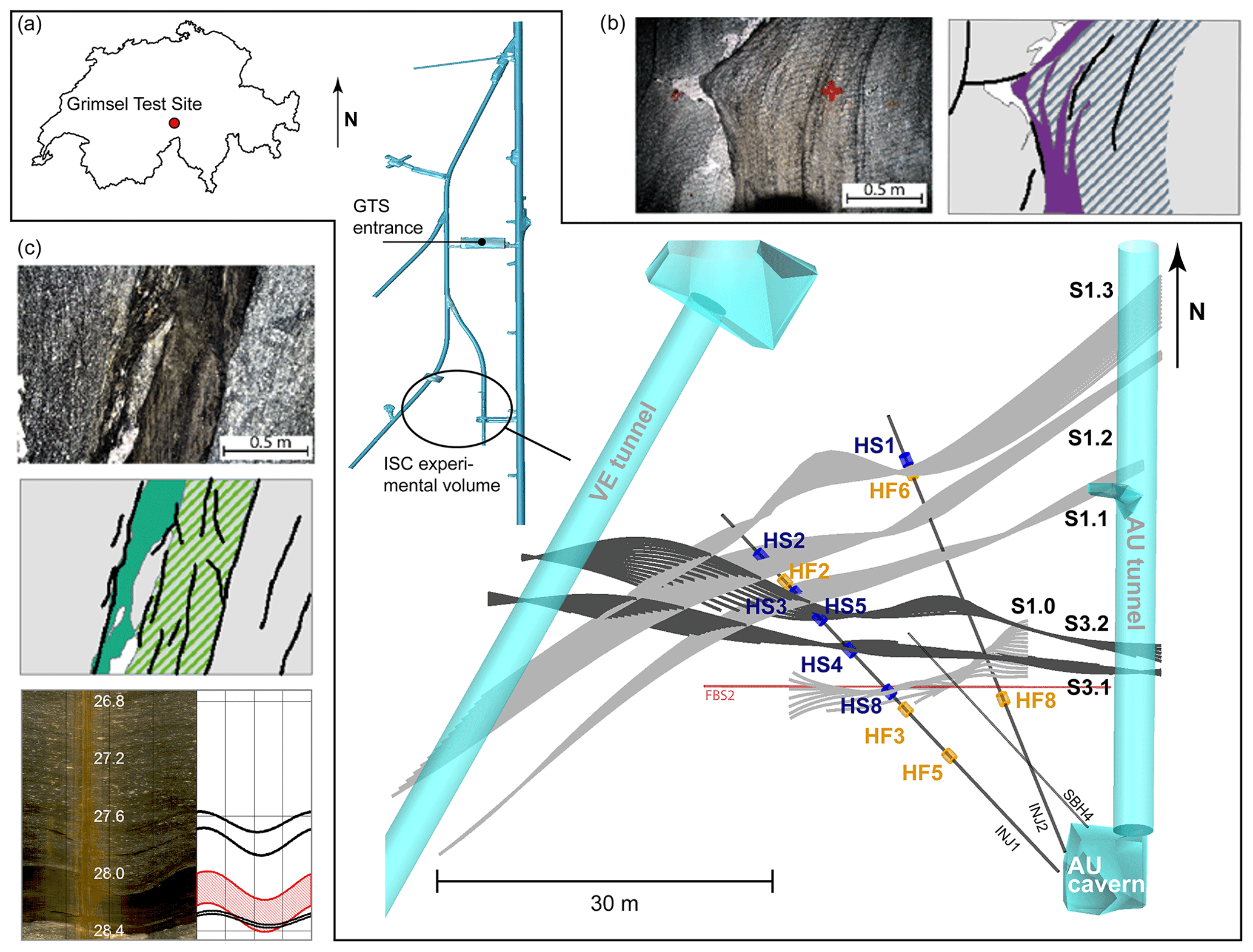
Figure 2(a) Location of the GTS in Switzerland (source: © https://www.d-maps.com/, last accessed: 23 April 2020) and the location of the ISC experimental volume in the tunnel network operated by Nagra, along with the top view of the ISC experimental volume located between the AU and VE tunnel. The two major shear zones S1 (gray) and S3 (black) intersect the experimental volume and the two injection boreholes (INJ1, INJ2) drilled from the AU cavern. The location of the HS (blue) and HF (orange) injection intervals are shown, as well as the strain-monitoring borehole FBS2 and stress measurement borehole SBH4 used in this study. (b) Shear zone S1 observed in the AU tunnel. (c) Shear zone S3 observed in the AU tunnel along with its observation in the injection interval (red and adjacent fractures in black) of experiment HS4. Panels (b) and (c) were modified after Krietsch et al. (2018a).
The GTS is located within the Central Aare massif, at the lithological boundary between Central Aare granite and Grimsel granodiorite. The rock mass in the test volume has a relatively low fracture density and a foliation with an average orientation of (dip direction/dip). Within the test volume, four shear zones with a ductile deformation history (referred to as S1 with an orientation of ) are characterized by a more distinct foliation compared to the host rock. These shear zones are associated with a few brittle fractures of various orientations that formed during retrograde deformation. In addition, two shear zones with a brittle–ductile deformation history (referred to as S3, ) are associated with biotite-rich metabasic dikes up to 1 m thick. The lateral distance between the two S3 shear zones is about 2.5 m, and the rock mass between the faults is heavily fractured with more than 20 fractures per meter in the eastern section of the test volume. The different shear zones were labeled with an increasing index number, counted from south to north (i.e., S3.1 is south of S3.2, which belong to the S3 group; Krietsch et al., 2018a).
The stress characterization revealed an unperturbed stress state (i.e., measured in a volume unperturbed by geological structures, about 30 m south of the S3 shear zone), with principle stress magnitudes of σ1=13.1 MPa, σ2=9.2 MPa, and σ3=8.7 MPa and dip direction/dip of (σ1), (σ2), and (σ3). The stress state close to the S3 shear zone is perturbed by geological structures, which results in changing principal stress magnitudes and orientations. The minimum principal stress decreases to 2.8 MPa, and the maximum principal stress direction rotates to 134/14∘ as the S3 shear zones are approached (Krietsch et al., 2018b). An overview of the mechanical material properties of the different species of granite found at the GTS is given in Selvadurai et al. (2019).
Six HS experiments were performed in February 2017, and six HF experiments were carried out in May 2017. Table 1 summarizes the details of each fluid injection in a chronological manner. The 12 injection intervals were chosen based on optical televiewer images taken in the two injection boreholes (INJ1, INJ2; Fig. 2) and the geological 3D model introduced by Krietsch et al. (2018a). For the hydraulic shearing experiments, four of the chosen intervals targeted S1 structures (Fig. 2, HS1, HS2, HS3, and HS8). Two injections were performed on S3 structures (HS4, HS5). The injection intervals had a length of 1 or 2 m and covered the target structure and adjacent brittle fractures (see example OPTV logs in Fig. 2b, c). The hydraulic fracturing experiments were performed in intervals without observable fractures. Three experiments were performed to the south of S3 (Fig. 2a, HF3, HF5, and HF8), and two experiments were performed north of S3 (HF1, HF2). The exception is the HF6 experiment, which was planned to be performed in a fracture-free interval but was conducted erroneously in a 1 m interval that contained S1.3 structures. Thus, the S1.3 structure stimulated during experiment HS1 was possibly re-stimulated during experiment HF6. Furthermore, during the initial injection experiment HF1, faulty shielding of a power line connecting the frequency control with the electric motor of the pump led to increased electronic interference on the seismic recordings and made further analysis impossible.
Table 1Overview hydraulic shearing and hydraulic fracturing experiments.
a Mean area of convex and concave hull. b,c Seismicity integrated to a magnitude of −9.
3.1 Injection protocol
A standardized injection protocol was used for the six HS experiments, to compare the influence of the targeted geological structures on the seismo-hydromechanical response. Roughly 1 m3 of fluid volume was injected per experiment (actual volumes are given in Table 1). The injection protocol consisted of four injection cycles (referred to as C1–C4, Fig. 4a), in which either the injection pressure or injection flow rate was increased in a stepwise manner after steady state was reached. All the cycles were followed by a shut-in phase, where pumping was stopped, and a venting phase, in which the pressure in the injection- and all monitoring-intervals were bled off. The first two pressure-controlled cycles C1 and C2 were conducted to determine pre-stimulation jacking pressure (i.e., the injection pressure at which the ratio between the injection pressure and flow rate deviates from linearity) and initial injectivity of the target structure. C3 was the actual flow-controlled stimulation cycle, in which the bulk part of the fluid was injected. C4 was initially pressure controlled, changing to flow-controlled injection, aimed at determining the post-stimulation jacking pressure and injectivity of the targeted structure. During all HS experiments, the flow rate did not exceed 38 L min−1.
HF experiments also followed a standardized injection protocol involving a target injected volume of ∼1 m3 (actual injected volumes in Table 1). The injection protocol for the five HF experiments started with a flow-controlled formation breakdown cycle (indicated by the letter F) to initiate the hydraulic fracture. This initial cycle and all the subsequent cycles included a shut-in phase were pumping was stopped. During some of the formation breakdown cycles the shut-in phase was complemented by a bleed-off phase of the injection interval and all pressure monitoring intervals. The two subsequent cycles were aimed at propagating the previously initiated hydraulic fracture (RF1, RF2). For these two propagation cycles, water was used during HF1, HF2, HF3, and for HF5, HF6, and HF8, shear-thinning fluid (xanthan–salt–water mixture, XSW) was used. We note that the XSW mixture exhibited a viscosity of ∼35 mPa s (viscosity of water =1 mPa s). Propagation cycles RF1 were performed with maximum flow rates of 35 L min−1. During experiments performed with water, the flow rate was controlled in a sinusoidal fashion (period: 2.5–20 s; amplitude: ±15 L min−1) for roughly 10 minutes. For experiments in which XSW was injected, an additional cycle, RF3, was added to inject water so that XSW is flushed from the fracture network. All the HF experiments were finalized by a pressure-controlled step-rate injection test (SR) for evaluating post-stimulation jacking pressures and injectivities of the created hydraulic fracture.
3.2 Seismic monitoring and data processing
3.2.1 Seismic monitoring
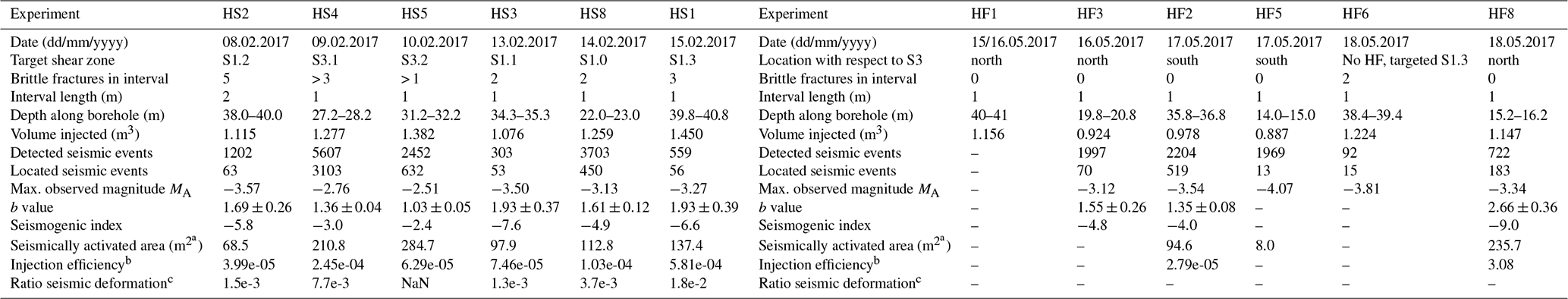
A total of 26 in situ acoustic emission sensors (AE sensors) formed the passive seismic network around and inside the test volume (Fig. 3a, green cones). The sensors were manufactured by the Gesellschaft für Materialprüfung und Geophysik GmbH (GMuG) and have a bandwidth of 1 to 100 kHz, with their highest sensitivity at 70 kHz. 14 AE sensors were installed on a tunnel level (R2–R15; type: Ma-Bls-7-70), in 55 mm diameter boreholes drilled approximately 250 mm deep into the tunnel wall. The bottom view AE sensors were pressed against the polished surface of the base of the borehole. The core of the network (i.e., sensors within 5–25 m distance to the injection intervals) was composed of eight borehole AE sensors (R16–R23; type: MA-BLw-7-70-68) distributed in four water-filled monitoring boreholes (GEO1–GEO4, Fig. 3a). The borehole AE sensors have a curved front surface and were deployed in sensor shuttles in which two pneumatic cylinders (line pressure 10 bar) ensured contact pressure between the sensors and the borehole wall. Four additional sensors (R24–R27; type: MA-BLw-7-70-86) with curved front surfaces were installed in borehole SBH4 (Fig. 2b). For calibration purposes, five one-component (1C) accelerometers (R28–R32; type: Wilcoxon 736T) were installed next to five of the tunnel level AE sensors (Fig. 3a, red cones, R4, R6, R7, R9, R11). The accelerometers were factory calibrated and feature a flat frequency response from 50 to 25 000 Hz, with a sensitivity of 100 mV g−1. They were mounted to brass disks (∅ 28 mm×1 mm), which were glued to the front surface of the 55 mm diameter and 100 mm deep boreholes drilled into the tunnel wall adjacent to the AE sensors (Fig. 3c). The seismic signals were recorded continuously on a 32-channel acquisition system at a 200 kHz sampling rate (GMuG, digitizer cards: Spectrum M2i.47xx). AE sensor channels had 1 kHz and accelerometer channels had 50 Hz high-pass analogue filters installed.
In addition to the passive seismic network, active seismic sources were installed; eight falling hammer sources were distributed in the AU and the VE tunnels. Two borehole piezoelectric sources were installed in borehole GEO2 and GEO4 (Fig. 3a, black arrows). The trigger signal of the seismic sources, used to determine the initiation time of each active seismic survey, was recorded on one channel of the acquisition system. The active sources were used for time-lapse 3D seismic tomography surveys during the experiments (see Schopper et al., 2020; Doetsch et al., 2018b, for details). For more information on the seismic monitoring system, see Doetsch et al. (2018b).
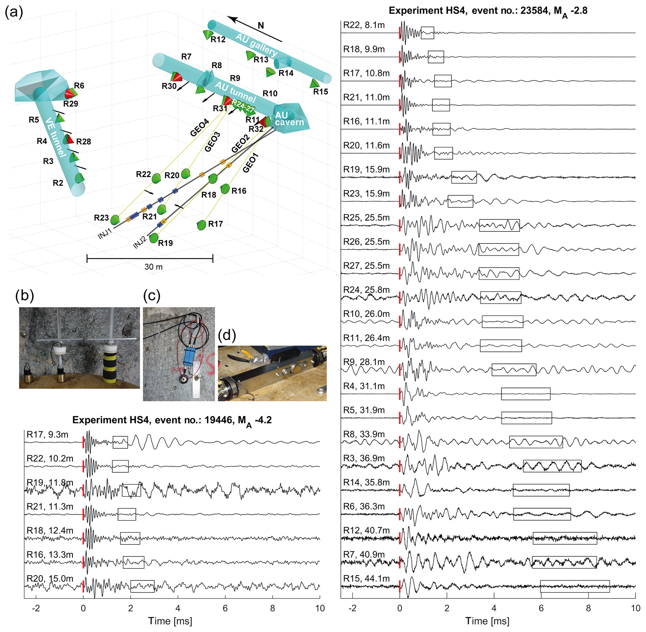
Figure 3(a) The seismic network consisting of 26 uncalibrated AE sensors (green cones) installed in four boreholes, the AU and VE tunnels, and the AU gallery, along with five one-component calibrated accelerometers (red cones) collocated with five AE sensors in the AU and VE tunnels. Seismic sources in the tunnels and boreholes are shown by black arrows. (b) AE tunnel sensor, insulated against acoustic noise. (c) Installed AE sensor next to a calibrated accelerometer along with their pre-amplifiers. (d) AE sensors in a sensor shuttle for deployment into water-filled boreholes. Waveforms from a small- and large-magnitude event induced during experiment HS4, including the Euclidean distance hypocenter−sensor, P-wave pick (red-stripe), and a window of a hypothetical S-wave arrival for an S-wave velocity of 2500–3000 m s−1 (applied bandpass filter for small event: 1–12 kHz; large event: 1–50 kHz).
3.2.2 Seismic data processing
Continuous recording of 32 channels at a sampling rate of 200 kHz with 16 bit digital resolution resulted in ∼250 GB of data over approximately 6 h of recording time. For flexible and fast access to the data, the Adaptive Seismic Data Format (ASDF; Krischer et al., 2016) proved to be adequate. The ASDF format is integrated in an open-source Python library for seismology (ObsPy) that was used for event detection.
For seismic event detection only the eight closest AE sensors to the center point of the injection interval were considered (i.e., R16–R23). Prior to any event detection, the data streams were bandpass filtered (fourth-order Butterworth filter) between 1 and 12 kHz. An ObsPy integrated detection algorithm with a recursive STA/LTA trigger and a coincidence threshold of two was used for event detection (i.e., a seismic event was declared when at least two detections of a potential seismic event were found). Many of the triggered events were electric noise interference characterized by their high-frequency and near-simultaneous occurrence on all channels. These events were automatically removed if the trigger time of the recursive STA/LTA algorithm or the time of the minimum or the maximum amplitude was within four sample points. The event catalogs produced with sensitive trigger settings were inspected visually to remove false events (e.g., electric noise, man-made signals produced in the tunnels, etc.). Note that throughout the experiments, active seismic surveys were performed approximately every 10 min. During the perturbance by the active seismic signals, i.e., 1 s for each hammer source and 35 s per piezoelectric source (TRBLw-1-86) burst, no passive event detection was performed (see also a detailed temporal evolution of seismic event detections, initiated active seismic signals, and injection parameters of all the experiments in the Supplement, Sect. S1).
P-wave onsets were manually picked for events with coincidence levels three to eight (i.e., the signal was detected on three to eight traces). As can be seen from the seismic events detailed in Fig. 3, S-wave signals were generally weak or undistinguishable. Thus, the S-wave onsets could not be picked and used for event location. Clear S-waves have been observed at comparable sites where similar monitoring equipment was installed (Kwiatek et al., 2011; Zang et al., 2016; Dresen et al., 2019). One reason why no S-waves are observed might be that the designed waterproof sensor shuttles, in which the borehole AE sensors were deployed, influence the ability to record S-waves.
3.2.3 Seismic event location
The seismic events were located using a homogeneous, transversely isotropic velocity model and standard inversion practice. The P-wave arrival times were weighted according to their P-wave pick uncertainties, which were estimated empirically as a function of signal-to-noise ratios (SNRs). The SNR was calculated from the maximum absolute P-wave amplitudes determined in a window defined by the P-wave onset and a theoretical S-wave onset (estimated with an S-wave velocity of 2800 m s−1), as well as the maximum absolute amplitude in a noise window taken in a window with the same length before the P-wave onset. At an SNR ≥30, P-wave pick uncertainties were estimated at plus/minus two samples; below a ratio of 30, P-wave pick uncertainties (in samples) were estimated with the following linear relationship:
The anisotropic velocity model is based on the weak elastic anisotropy formulation of Thomsen (1986). Thomsen's formulation for transverse isotropy is
where vP is the P-wave velocity along a respective ray path, vP,sym represents the P-wave velocity along the anisotropy symmetry axis (i.e., usually the minimum velocity), θ is the angle between the symmetry axis and the ray path, the parameter ε represents the relative increase in velocity perpendicular to the symmetry axis, and δ describes the angular dependency of the velocity. The best-fitting anisotropic velocity model (i.e., vP,sym, ε, δ, azimuth, and dip of symmetry axis) was inferred with a MATLAB genetic algorithm from a sub-catalog of 495 induced high-quality seismic events exhibiting more than nine P-wave picks and locations distributed over the entire experimental volume. For this, the median of the root mean square (RMS) of the differences between theoretical and observed arrival times for 495 high-quality event locations was minimized. Furthermore, to verify the estimated P-wave pick uncertainties, the dimensionless χ for each of the 495 events in the sub-catalog was computed and did not exceed a value of 3.6.
Note that the target value for χ is 1.0, for which the discrepancy between the observed and predicted arrival times is equal to the estimated pick uncertainty. Values above 1.0 suggest an underfitting, while values below 1.0 suggest an overfitting of the data.
Comparing the velocity parameter determined through the aforementioned analysis steps, with the seismic velocity parameter introduced by Gischig et al. (2018) at similar location at the GTS, our inferred seismic velocity in the direction of symmetry, vp,sym, is about 5.5 % lower, but the ratio between the two velocities, ε, remains the same. A slight change in the angular velocity dependency, δ, was also observed (0.07 instead of 0.02). The dip direction and dip of the symmetry axis also changed slightly compared to Gischig et al. (2018) ( instead of ). We attribute these differences to the geological conditions; the rock mass contained a highly fractured shear zone compared to the less fractured rock mass within the ISC test volume targeted by Gischig et al. (2018) for mini-fracturing experiments. Station corrections were determined for each sensor location using the joint hypocenter determination (JHD) approach analogous to Gischig et al. (2018). The JHD approach simultaneously optimizes hypocenter locations of the 495 sub-catalog events and systematic shifts in travel times arising from error in sensor locations or geological conditions around the sensor.
To estimate location uncertainties in source locations due to pick uncertainties, the arrival times were randomly perturbed 1000 times with the estimated pick uncertainties of Eq. (1) (similar to Gischig et al., 2018). The principal directions and dimensions of the point clouds consisting of the 1000 new locations were analyzed to estimate the location relative errors. Only events with the largest error axis below 3 m (i.e., ±1.5 m) were analyzed further.
Absolute location uncertainties were estimated by comparing the known initiation locations of high-energy sparker shots (i.e., high-voltage electric discharge, which triggers a compressional wave in formation water-filled boreholes) in injection boreholes and their inferred location through the determined velocity model and station corrections. The absolute location errors were below 0.5 m in injection borehole one (INJ1) in an interval from 15 to 30 m depth and increased to around 1.5 m towards the borehole top and bottom. For injection borehole two (INJ2) the absolute error was below 1 m in an interval from 15 to 30 m depth and increased to around 1.5 m towards the borehole mouth and bottom.
3.2.4 Magnitude computation
In this section three different magnitudes are computed, including (1) a maximum P-wave-amplitude-based Mr for the entire catalog, corrected for angle-dependent sensitivity variations and variation in coupling quality. Mr's are relative magnitudes as they were determined from amplitudes of uncalibrated sensors. (2) For some strong events moment magnitudes Mw were derived. (3) An amplitude magnitude MA adjusted to a realistic magnitude level was then computed for the entire catalog using a linear relation between Mr and MA. The relation was derived by comparing Mr and Mw for which an Mw was available.
Generally, determining the magnitude of seismic events recorded on uncalibrated AE sensors is challenging. Angle-dependent sensitivity variations and varying coupling quality make it impossible to infer a simple and universal instrument response (Kwiatek et al., 2011). However, to characterize the relative source strength of induced seismic events, relative magnitudes, Mr, were estimated from the maximum P-wave amplitudes of uncalibrated AE sensors in the time domain following the approach introduced by Eisenblätter and Spies (2000) in combination with an attempt to account for angle-dependent sensitivity variations and variations in coupling quality. To adjust the estimated relative magnitudes Mr to a realistic magnitude level, the absolute magnitudes Mw are determined for events recorded on tunnel-level AE sensors collocated with calibrated accelerometers (Fig. 3a, red cones). Adjusted relative magnitudes Mr are referred to as amplitude magnitudes MA. Relative magnitudes were estimated as follows:
where Ai is the bandpass-filtered (3–12 kHz) maximum P-wave amplitude determined in a window confined by the P-wave arrival pick and a theoretical S-wave arrival, assuming a shear wave velocity of 2800 m s−1. ri is the source-sensor distance; r0 is a reference distance (chosen to be 10 m), and N is the number of P-wave arrivals of the respective event. represents the frequency-dependent attenuation coefficient, where f0 is the dominant frequency, which was chosen to be the middle frequency of the filtered band (i.e., 7.5 kHz), Vp is the P-wave velocity, and Qp is the quality factor representing seismic attenuation. Qp was measured at the GTS by Holliger and Bühnemann (1996) in a frequency range of 50–1500 Hz and was reported as 20–62.5. More recently, Barbosa et al. (2019) estimated Qp from full-waveform sonic data in the injection boreholes using sources in the range of 15–25 kHz. They found QP=13 on average with a drop to the very low values of 8 in the vicinity of the metabasic dikes and the shear zones. Based on these observations, we chose a Qp value of 30. For the relative magnitude estimate, only tunnel sensors (R2–R15) and borehole sensors (R16-R23) were used.
(a) Correction of angle-dependent sensitivity variation of AE sensors
The installed AE sensors at Grimsel are of similar type to the AE sensors used by Manthei et al. (2001), who observed a declining sensitivity with an increasing incidence angle of incoming seismic waves with respect to the sensor normal. The varying sensitivity is due to both the design of the sensor and the coupling quality of the sensor to the rock and thus cannot be dealt with in a generic manner, as is described by GMuG. The influence of the incident angle (i.e., the angle between the direct ray and the sensor normal) on the relative magnitudes of the incoming seismic waves has been characterized experimentally at the GTS using the two parallel boreholes GEO1 and GEO3 (Fig. 3a). A piezoelectric source of the type TR-BLw-1-86 (manufactured by GMuG) was incorporated in the same shuttle as the AE sensors, radiating seismic energy in a spectrum similar to the observed seismic events (1 to 15 kHz). The sensor was deployed in GEO3 at a fixed location and facing in the direction of GEO1, while the source was placed in GEO1 and moved in 0.5 m increments, resulting in an incidence angle range from 0 to 50∘. The waveforms of 250 pulses per location were stacked. From these signals, a relative magnitude Mr was estimated revealing a linear decay of Mr as the incident angle increased (see Sect. S2, panel a). Averaging the slope of 20 measurement series at 20 different locations along the boreholes GEO1 and GEO3 and accounting for any variation in coupling quality leads to an angle-dependent Mr correction function , where Mr is the relative magnitude estimated without correction, and α is the incident angle of the direct incoming P-wave. Note that because we are lacking knowledge of the decline of sensitivity of AE sensors above a 50∘ incidence angle, Mr was only estimated at AE sensors for which the incidence angles did not exceed 50∘.
(b) Correction for variation in coupling quality of AE sensors
To account for variations in the coupling quality of AE sensors during the actual stimulation experiments, a correction quantity was calculated for each AE sensor by iteratively minimizing the median of sensor residuals as follows:
where is the median difference in the ith sensor, is the mean relative magnitude of at least three sensors, and is the relative magnitude estimate of the ith sensor (see Sect. S2, panel b).
After the application of the aforementioned corrections, standard deviations of the estimated Mr are, for most of the seismic events, approximately 0.3 but can reach 0.7. Standard deviations are lower for events located in the focus of the seismic network (i.e., experiments HS4 and HS5).
(c) Estimating instrument responses for AE sensors
In order to establish the absolute magnitudes Mw for a subset of located events, we determined the instrument responses for the five collocated AE sensor–accelerometer pairs installed on a tunnel level using the spectral deconvolution calibration technique introduced by Plenkers (2011) and Kwiatek et al. (2011). Based on their technique a calibration function, Z(f), can be computed by
where uAE(f) and uAcc(f) represent the displacement signals, and iAE(f) and iAcc(f) are the instrument responses in the frequency domain of the acoustic emission sensors and the calibrated accelerometers, respectively. From the complex calibration function Z(f), only the modulus of the relative amplitude calibration function |Z(f)| is used. The calibration technique relies on seismic signals recorded on both the AE sensors and the collocated calibrated accelerometer. However, most of our induced seismic events were too weak to be recorded by the less sensitive accelerometer with adequate high-frequency quality. Therefore, instrument responses were inferred from the aforementioned high-energy sparker shots performed every 0.5 m in the boreholes INJ1, INJ2, and GEO1–4 (Fig. 3a). Sparker shots radiate seismic energy in a similar frequency band as the induced seismic events (∼1–50 kHz).
To infer instrument responses, 4 ms of the waveform centered around the first P-wave arrival from performed sparker shots were used (excluding clipped signals and signals with an SNR ratio smaller than 10 dB). Before computing the Fourier spectra, the waveforms were bandpass filtered (AE sensors: 1–50 kHz; accelerometer: 1–25 kHz), zero padded and tapered with a Hanning window. Signal and noise spectra were smoothened using a Savitzky–Golay filter (polynomial order: 3; frame length: 51). The maximum frequency considered for the instrument response is the one that still had a signal 3 dB above the noise floor.
Instrument responses were calculated for 10 sparker shots per incidence angle bin of 15∘ up to incidence angles of 60∘, since it was suggested by Kwiatek et al. (2011), Plenkers (2011), and Naoi et al. (2014) that the instrument responses are incidence angle dependent. However, no angle dependency could be resolved for our sensor pairs, perhaps because both the AE sensors and 1D accelerometer were oriented in the same direction and the angle-dependent sensitivity variations canceled out. We note that, compared to the studies that showed sensitivity variations with changing incidence angles, the incidence angle of seismic events in our study (i.e., sparker shots in our case) differed in spatial scale. In this research, we were limited to a rather narrow band and did not exceed 60∘ because the AE sensor–accelerometer pairs installed at the tunnel level were aligned towards the injection intervals (see the geometric details shown in Fig. 3a). Since we did not observe angle-dependent variations in the instrument responses, we used the 10 instrument responses that exhibited the largest frequency range and found no difference in the incident angle of the direct P-wave. In contrast to the incidence angle dependency of instrument responses, distinct variations in instrument responses for the different collocated AE sensor–accelerometer pairs were observed (see Sect. S2, panel c), which is possibly due to different coupling qualities of the sensors. Thus, it is impossible to transfer instrument responses for other AE sensors installed at the tunnel level to those down borehole. We have therefore only calculated the absolute magnitudes Mw as determined for the AE sensors (R4, R6, R7, R9, and R11) collocated by the accelerometers (R28–R32).
(d) Estimating absolute magnitudes Mw for a subset of events
For corrected P-wave source spectra recorded on AE sensors R4, R6, R7, R9, and R11 exhibiting a SNR > 10 dB, moment magnitudes were determined by fitting the theoretical displacement source spectrum introduced by Boatwright (1978), corrected for aseismic attenuation and geometrical spreading to the observed spectra, as follows:
where Ω0,P is the low-frequency plateau of the P-wave spectrum, fc represents the corner frequency, QP is the frequency-independent quality factor (again set to 30), and vP represents the P-wave velocity (chosen to be 5030 m s−1; mean anisotropic velocity); R is the source–sensor distance. The scalar seismic moment is then derived from the low-frequency plateau using
Here, ϱ represents the density of the rock mass and is chosen to be 2650 kg m−3; the radiation pattern correction factor, RP, is set to 0.52, and the free-surface correction factor, ΥP, is chosen to be 2 (Aki and Richards, 2002). The scalar seismic moment is converted into a moment magnitude using the relation . The theoretical spectrum ΩP was fitted to the observed spectrum using a grid-search varying M0 and fc, keeping QP constant. Mw's were estimated for events with at least two Mw estimates. Comparing the obtained Mw with Mr leads to the relationship for the amplitude magnitude (see Sect. S7).
In the following, we present and compare seismicity observed during the ISC stimulation experiments. Seismicity is in one case combined with strain observations in the experimental volume, in order to show the diversity and interaction of the observed properties (Sect. 4.2).
4.1 Temporal seismic event evolution
For the HS injection experiments, most events (12 211 from a total 13 826 detections) were detected during pumping phases (Fig. 4a, b, for a selection of HS experiments). The percentage of events recorded during shut-in were in the range of 10 %. Less than 2 % of events were detected during venting. Comparing the HS experiments, significantly fewer events were detected during experiments at the S1 shear zones compared to the stimulation experiments performed at the S3 shear zones (Table 1). An exception was HS8 at the S1 shear zone south of S3, which produced a number of events comparable to the S3 injections (i.e., total detections: 3703). This may be explained by the fact that the injected fluid entered the S3 shear zone, which was evident from the seismicity cloud migrating towards the S3 shear zone (see Sect. 4.2). The number of seismic events (normalized to the total number of events per experiment) is plotted against injected volume in Fig. 5a and b. Again, a distinct behavioral difference between S1 and S3 injections is observed. During experiments in S1, the largest seismic detection rate was observed during stimulation cycle 1; more than 50 % of all events were induced with less than 100 L of fluid (< 10 % of the total volume). On the contrary, for S3 stimulations, most events were detected during cycle 3, when the largest volume of fluid was injected. Again, experiment HS8 is an exception in that the highest detection rate was observed during cycle 1 (similar to S1 stimulations), after which the event rates behave similarly to the S3 injections (HS4, HS5). Generally, a larger fraction of seismic events occurred after shut-in during injection into the S1 shear zones compared to injections into the S3 shear zones.
Over all HF injections, about half of the detections were made compared to the HS injections (see Fig. 4c, d, for a selection of HF experiments). Most of the events were detected during the pumping phases (4483 of 6731 detections). Interestingly, a comparably high percentage of detections (33 %) were made during shut-in, and no events were detected in the venting phases. We argue that the high percentage of post-shut-in detections were related to a hydraulic connection created between the injection interval and the open seismic monitoring boreholes (termed GEO) during the last two experiments HF5 and HF8. This hydraulic connection allowed observable flow from the GEO boreholes into the tunnel. We assume that this flow triggered stick-slip movements of the AE sensors. Thus, ongoing flow through GEO boreholes after shut-in would explain why many post-shut-in events were detected. Also, most of these events were only detected at the two sensors in the GEO borehole which was hydraulically connected. Note that HF6 – by mistake placed across the S1.3 shear zone close to the injection interval of HS1 – can be seen as a continuation to the HS1 experiment.
In summary, for the HS experiments, 31 % (i.e., 4342) of detected events could be located. The fraction of located shut-in events during the HS experiments is around 3 %, the fraction of events induced during the venting phase is less than 1 %. For the HF experiments, because of the large number of events without seismic origin (possibly sensor stick-slip), only 12 % (i.e., 781) of all detected events could be located. Six percent of the events were located after shut-in, and no events were located during the venting phases. The located seismic events fulfill a location uncertainty below ±1.5 m (for more information on location uncertainty see Sect. 3.2.3).
The maximum induced magnitudes Mmax during both HS and HF experiments (see inset of Fig. 1 and yellow stars in Figs. 4 and 5) occurred during pumping with no evidence of a temporal trend. Events during a time interval between shut-in and the start to a new injection cycle were usually of lower magnitude. One exception was the injection experiment HF6; here the highest-magnitude event was induced during a shut-in phase (see Sect. S3).
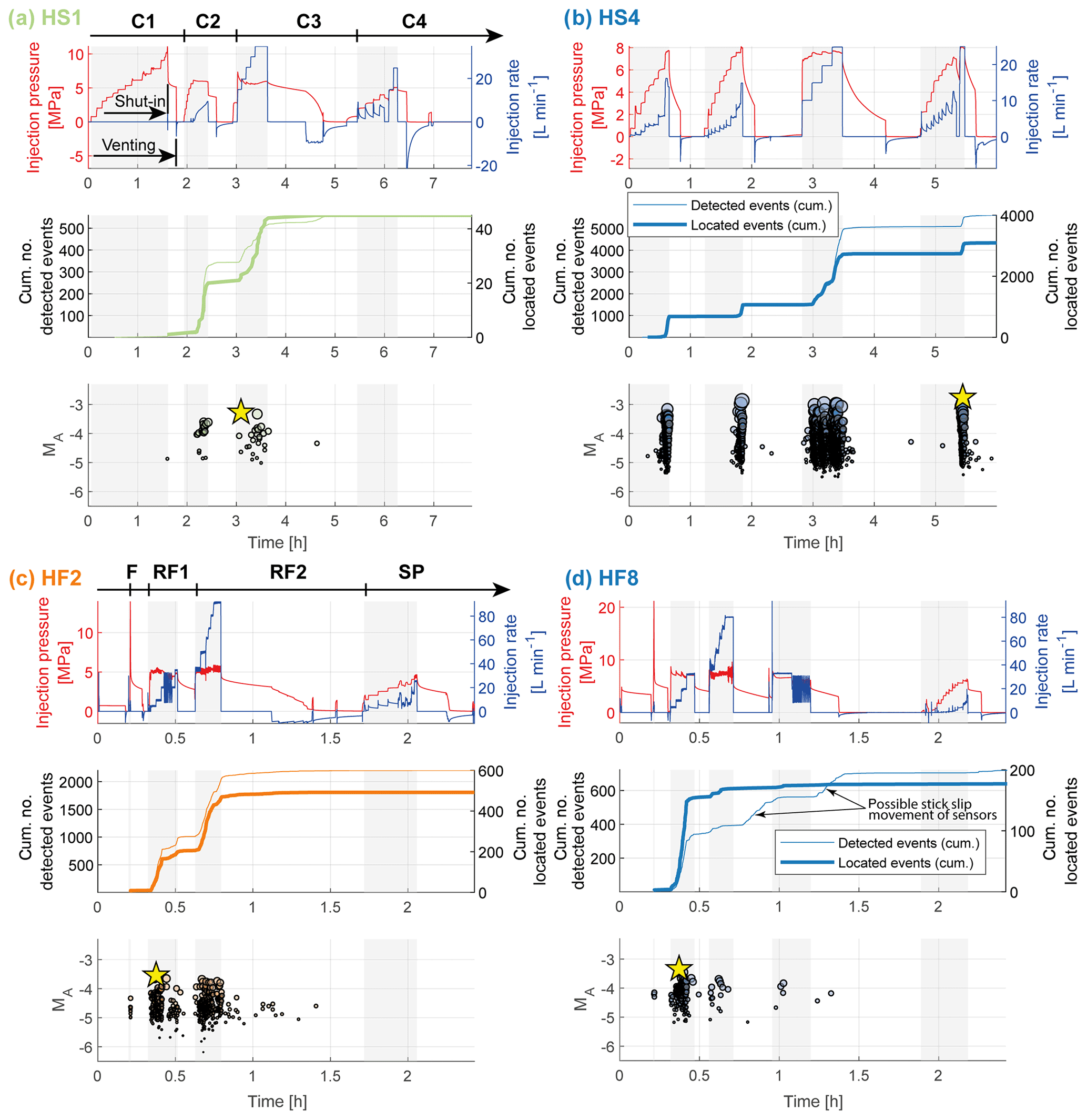
Figure 4(a) Temporal seismicity evolution of experiment HS1 performed in shear zone S1.3 and (b) of experiment HS4 in shear zone S3.1, along with (c) the temporal seismicity evolution of experiment HF2, which was performed north of the S3 shear zones, and (d) the temporal seismicity evolution of experiment HF8, performed south of the S3 shear zones. In addition to the injection rate and pressure, the cumulative number of events and magnitudes MA are shown. The largest-magnitude event is indicated with a yellow star. The shaded area on the plots indicate the pumping periods during an experiment (the temporal seismicity evolution of the remaining experiments is shown in Sect. S3, of this paper). Panel (a) also shows an example for a HS injection protocol with injection pressure and injection flow rate, divided into the four cycles, including shut-in and venting phases in each cycle. Panel (c) shows an example of a HF injection protocol with injection pressure and injection flow rate, including formation break down cycle (F), refrac cycles (RFs), and the final step pressure (SP) injection experiment. All of the cycles include a shut-in phase, but only after some cycles a venting phase is included. The yellow stars indicate the largest events induced in a respective experiment.

Figure 5Cumulative fraction of detected events as a function of cumulative injected volume of (a) HS and (b) HF injection experiments. Panels (c) and (d) show absolute values of located events above a magnitude level of MA −4.02 (maximum MC in the experimental volume; see Sect. 4.3) for HS and HF experiments, respectively. Note that for experiment HS3 only one event was observed above the maximum MC in the experimental volume and is thus not shown in Fig. 5c.
4.2 Spatial properties of seismicity clouds
4.2.1 Spatial distribution
The seismicity clouds produced by the HS experiments (Fig. 6a, c) form planes with a tendency to align in the E–W direction (main direction of S3 shear zones) or in a NE–SW direction (main direction of S1 shear zones). Often these planes exhibit substructures with events grouped into clusters, which is most pronounced for experiment HS4 (see also Figs. 7 and 8). Note that we use the term “cluster” here for a distinct subgroup of seismic events within the seismicity cloud of individual experiments. These are not clusters derived from waveform similarity and relative relocation, which is the scope of future studies. The seismicity induced by the injection experiments in injection borehole INJ1 predominately propagated in an easterly direction, whereas the seismicity cloud of HS1, the only HS injection in INJ2, was oriented in a NE–SW direction (Fig. 6a). For this experiment the seismicity occurred exclusively a few meters above the injection interval (Fig. 6c). For HS8, the injection experiment closest to the top of injection borehole INJ1, there was a tendency for downward propagation. Generally, seismicity is well contained within narrow clouds surrounding the injection interval. However, interactions (i.e., hydraulic or mechanical) were evident in experiments HS4 and HS8, where part of the HS8 seismicity cloud aligns with the HS4 seismicity cloud.
The seismicity clouds of the HF injection experiments also had a tendency to propagate in the E–W direction, similar to the HS experiments. Experiments conducted in INJ1 (i.e., HF2, 3, 5) induced seismicity clouds that propagated towards the east from the injection interval, whereas injection into INJ2 (i.e., experiment HF8) induced a seismicity cloud propagating towards the west (Fig. 6b). HF6, the HF experiment misplaced at the S1.3 shear zone, induced only a few seismic events superimposed on the seismicity cloud of experiment HS1 that targeted at the same structure. Seismicity clouds that occurred during the HF experiments propagated preferentially downwards. Injection experiment HF3 stands out in that it induced a dispersed seismicity cloud, with seismic events located at sites where previous experiments (i.e., experiments HS8 and HS4) had already induced seismicity, possibly indicating interaction with the HS8 and HS4 stimulated zones. Thus, no main cloud with a distinct orientation could be identified for experiment HF3.
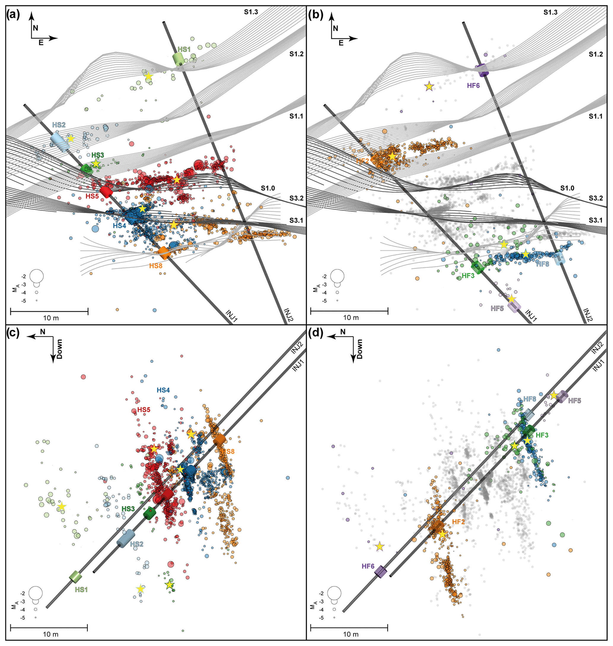
Figure 6(a) Overview of HS event locations in top view including interpolated shear zones and (c) side view towards east and (b) overview of HF event locations in top view including interpolated shear zones and (d) side view towards east. Injection intervals and seismic events of respective experiments are color coded. The maximum magnitude of each stimulation experiment is indicated with a yellow star. The gray events in (b) and (d) show the seismic events induced during the HS experiments, which were performed prior to the HF experiments. Note also that in order to improve visibility, the diameter of the injection intervals is exaggerated.
Planes fitted through the seismic event clouds by orthogonal distance regression are shown in Fig. 7 as half-circles and their poles in lower-hemisphere stereographic projections. The standard deviation of orthogonal distances of the seismic event locations to the fitted planes is below ±1 m, except for experiment HS1 (standard deviation ±1.4 m). The poor plane-fit quality for HS1 events may be associated with increased location uncertainty at the bottom of injection borehole INJ2 (see Sect. 3.2.3).
For injections HS1, HS2, HS3, HS5, HF5, and HF8, single seismic clusters were observed and fitting a single plane proved to be sufficient. Three seismic clusters were observed in injection HS4, and in injection experiment HS8 and HF2 two seismic clusters were observed. Planes were fitted to each of these clusters (Fig. 7). No plane was fitted to experiment HF3 due to the dispersed character of its seismicity cloud. For experiment HF6, there were too few located seismic events (details of the fitted planes can be found in the Sect. S4).
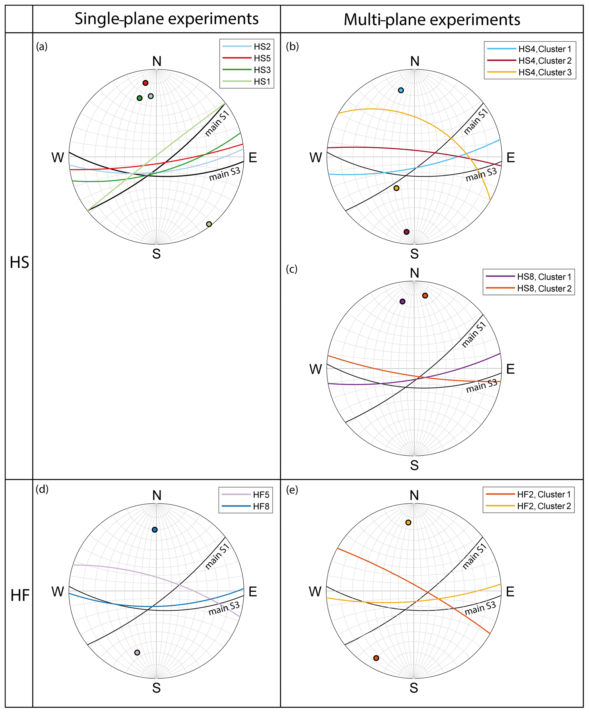
Figure 7Orientation of fitted planes and corresponding pole points through seismic clouds in lower-hemisphere stereographic plots, including main orientations of shear zones S1 and S3 observed in the tunnels. Plots are as follows: (a) for HS1, 2, 3, and HS5 for which a single-planar orientation of stimulation was identified; (b) for the three visually identified seismic clusters of injection HS4; (c) for the two clusters of injection experiment HS8; (d) for HF5 and HF8, for which a single and planar orientation of stimulation was identified; and (e) for the two visually identified seismic clusters of injection HF2.
Also included in Fig. 7 are the main orientations of the S1 and S3 shear zones observed in the surrounding tunnels (Krietsch et al., 2018a). Interestingly, the seismicity clouds of experiments HS2 and HS3, both targeting S1 structures, have an orientation similar to HS5 and to the main orientation of the S3 shear zones. Only the seismicity cloud of the S1 stimulation HS1 is oriented similarly to the main orientation of S1 shear zones, although its dip is slightly steeper. The HS4 seismicity produced three distinct cluster orientations: Cluster 1 formed from the injection interval and propagates sub-vertically in the ENE direction; Cluster 2 formed higher up in the injection interval and was oriented E–W, parallel to the shear zone S3.1; and Cluster 3 is a new fracture that formed during the main stimulation cycle (C3). The fracture formed at a location that was deemed to be fracture-free during geological characterization prior to the stimulation experiments. In addition, the formation of the new fracture was observed as a strong and abrupt opening by a 1 m long strain-monitoring sensor installed in a borehole (i.e., FBS2; see also Fig. 2) parallel to the S3.1 shear zone (Fig. 8d). For more information about the strain monitoring system see Doetsch et al. (2018a) and Krietsch et al. (2020). The strong tensile signal from the strain-monitoring interval at the 24 m borehole depth and the contraction of the adjacent strain-monitoring intervals began when there was a step rate increase in fluid flow. The opening lasted for about 10 min and was accompanied by the HS4 seismicity Cluster 3. Peak extensional strain occurred at shut-in. Contraction of the fracture during the shut-in phase is also associated with seismicity, after both cycles 3 and 4.
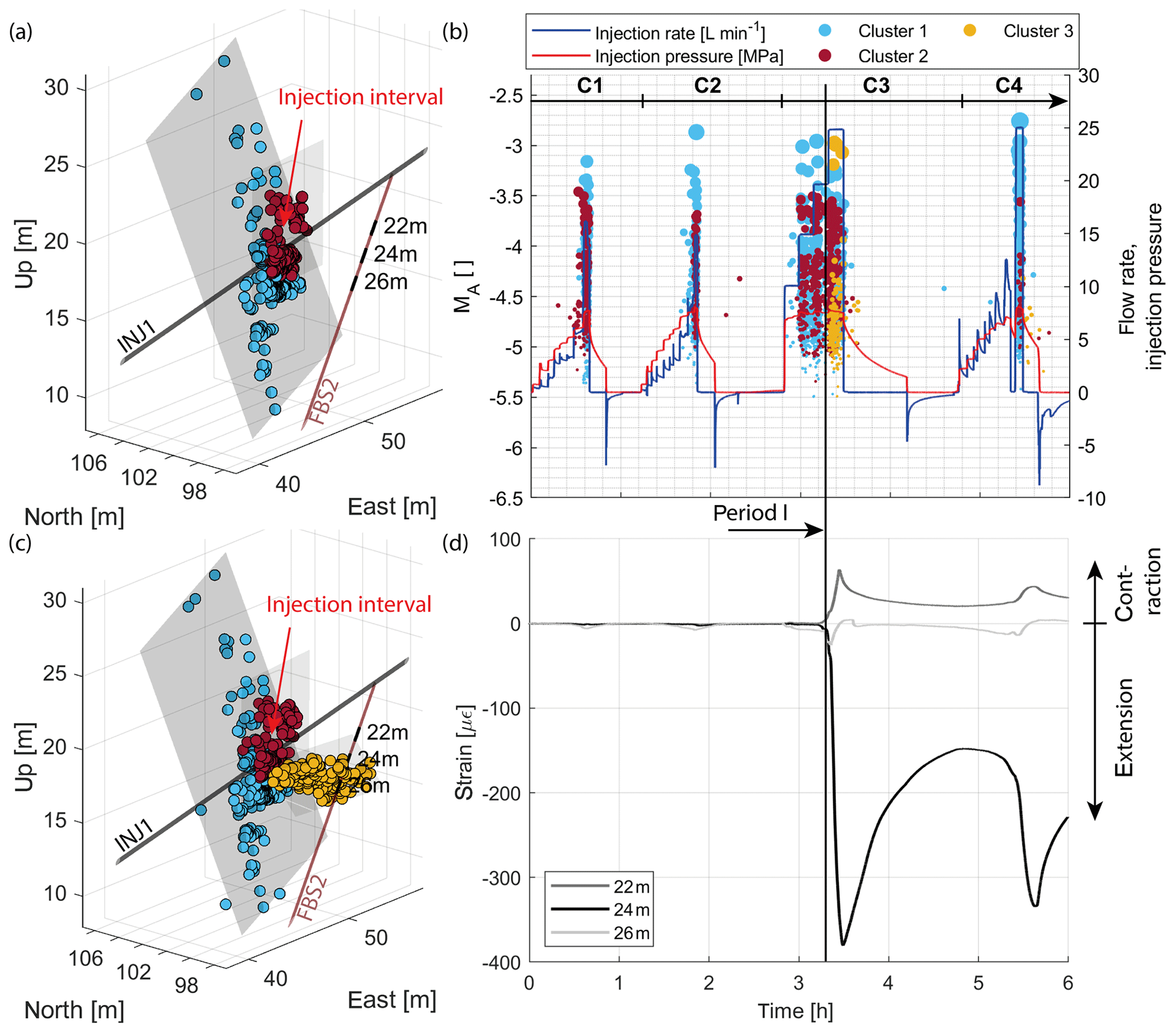
Figure 8Observation of newly formed fracture during injection experiment HS4. (a) The spatial distribution of seismicity clusters observed during period I, color coded according to cluster affiliation, along with injection borehole INJ1 and the strain-monitoring intervals at 22, 24, and 26 m in the strain-monitoring borehole FBS1. (b) The temporal evolution of seismicity including injection parameters. (c) Spatial distribution of all seismicity of the three main clusters. (d) The strain evolution of strain-monitoring intervals at the specified depths.
The two clusters of experiment HS8 indicate an initial stimulation of shear zone S1.0 in the ENE direction, hydraulically connecting the injection interval with injection borehole INJ2. The second seismicity cluster indicates stimulation along lower regions of shear zone S3.1 in the E–W direction, possibly because the zone stimulated during experiment HS4 was reactivated during HS8.
The seismicity cloud from experiment HF8 is oriented E–W, again comparable to the orientation of S3, while the seismicity cloud of HF5 deviates from this orientation. Experiment HF2 contains two main seismicity clusters: Cluster 1 includes the events propagating from the injection interval and is oriented comparable to the orientation of HF5. With ongoing stimulation, Cluster 2 is formed and orients itself in the E-W direction.
4.2.2 Propagation of seismicity
Over all injection experiments, a maximum distance of 20 m between seismic events and respective injection intervals was observed. For experiments targeting S1 shear zones, located events in the early cycles (C1, C2) cover more than 80 % of the maximum distance to the injection interval. Diffusivity values over all experiments are in the range of to m2s−1, with S1 stimulation experiments tending towards higher diffusivities. These values are almost 1–2 orders of magnitude smaller than diffusivity values observed in field-scale stimulations (Fenton Hill: 0.17 m2 s−1; Soultz: 0.15 m2 s−1; Basel: 0.06 m2 s−1; Dinske, 2011). Diffusivity values were estimated using the concept of seismic triggering fronts in a homogeneous, isotropic, and poroelastic medium introduced by Shapiro et al. (2002) with the awareness that the concept disregards varying fluid injection rates, which have an effect on seismicity propagation (Schoenball et al., 2010). For more information on the diffusivity estimates we refer to Sect. S6.
We further investigated the 2D seismicity propagation along the reactivated fractured zones by projecting the seismic event locations for each experiment onto the best-fitting planes (experiment and injection cycle resolved projections can be found in Sect. S5). In general, only a few experiments (e.g., HS8 and HS4) show concentric growth of seismicity. Seismicity of subsequent cycles often occurs at the same location, which suggests that the same fracture zones are reactivated during repeated injection. Furthermore, the seismicity of many of the injection experiments shows a change in propagation direction for repeated cycles (HS1, HS2, HS3, and HS5; for experiment HS5 see also Krietsch et al., 2019).
4.3 Frequency–magnitude distributions
The Gutenberg–Richter a and b values are estimated for partial catalogs of respective injection experiments defined by the magnitude of completeness, MC. The latter was determined per experiment using the goodness of fit method introduced by Wiemer and Wyss (2000). a and b values and their uncertainty are calculated using the modified maximum likelihood technique published by Marzocchi and Sandri (2009). a values are normalized by the injected volume to derive the so-called seismogenic index, Σ (Dinske and Shapiro, 2013). Figure 10 shows frequency–magnitude distributions (FMDs) of all injection experiments. MC and a and b values were estimated for injection experiments exhibiting more than 20 seismic events and a goodness of fit quality of more than 90 %. Exceptions were made for injection experiment HS3 and Cluster 3 of experiment HS4, where the goodness of fit quality lies above 85 %. MC is lowest for injections in the focal point of the seismic network (HS4: −4.90; HS5: −4.80; HF2: −4.78). For injection experiment HS4, a bimodal frequency–magnitude distribution was observed. For a and b value calculations, the higher MC of −4.32 was used. MC increases for injections performed outside the network focus (HS3: −4.66; HS2: −4.39; HS8: −4.38) and is highest for the injection experiments performed towards the bottom of the second injection borehole (INJ2, HS1: −4.05) and towards the tops of the two injection boreholes (HF3: −4.14; HF8: −4.02;see Fig. 9). Thus, for these experiments the range between the maximum induced magnitude and MC is small. Moreover, when investigating spatial and statistical properties of seismicity clouds one has to be aware of the spatially varying network sensitivity. Our eight borehole AE sensors close to the injection intervals are decisive for an increased network sensitivity in the experimental volume close to the injection boreholes. In addition to the source–receiver distance, the sensitivity of the network is significantly influenced by the directivity of the AE sensor; i.e., events with incident angles > 50∘ in the Grimsel experiment are less likely to be detected.
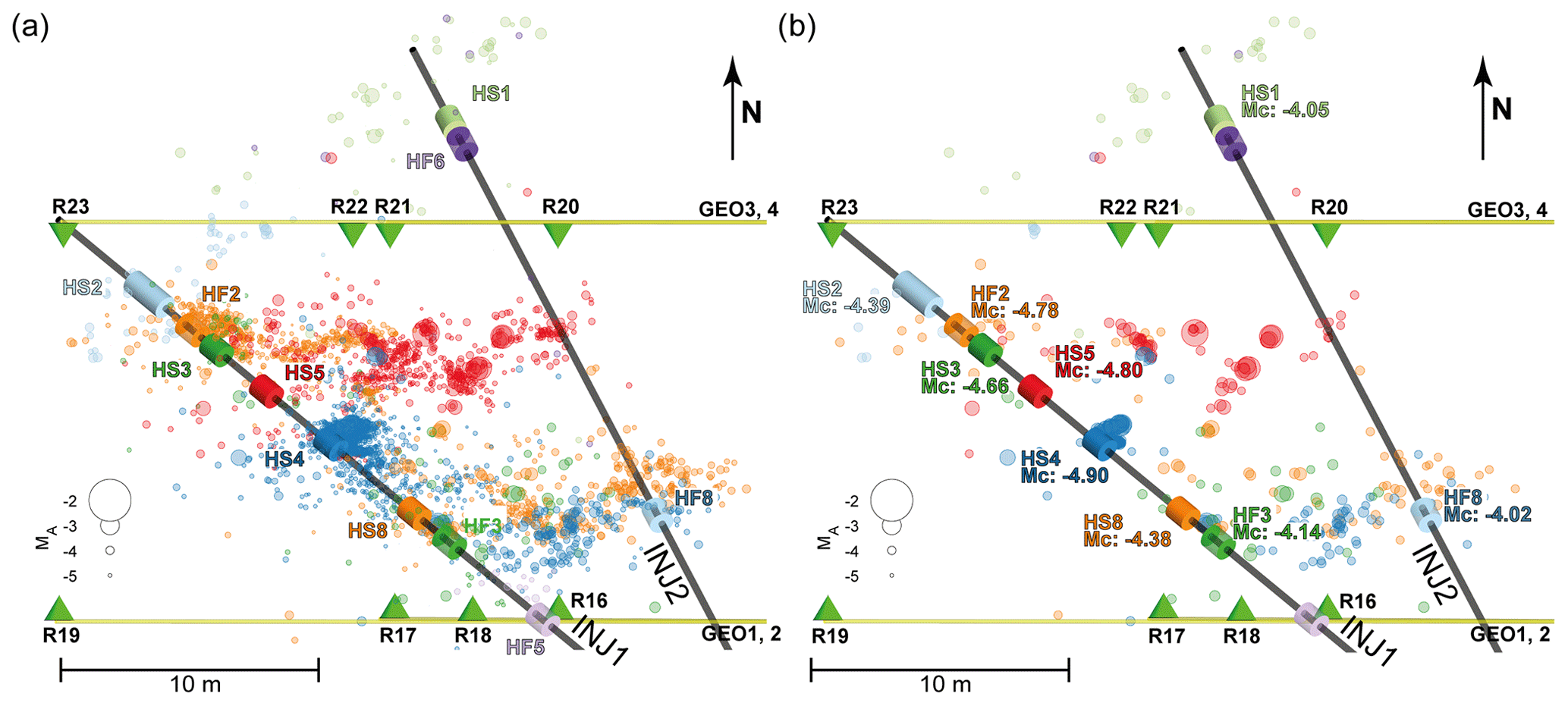
Figure 9Top view comparison of (a) all located seismic events with (b) seismic events exhibiting magnitudes above the maximum encountered MC in the experimental volume (i.e., MC−4.02) along with MC estimates of experiments, injection boreholes, injection intervals, and borehole AE sensors.
The HS injection experiments (Fig. 10a) targeting S1 shear zones exhibited larger b values (HS1: 1.93±0.39; HS2: 1.69±0.26; HS3: 1.93±0.37) and lower seismogenic indices (HS1: −6.6; HS2: −5.8; HS3: −7.6) compared to the b values of injections into S3 shear zones (HS4: 1.36±0.04; HS5: 1.03±0.05) with higher seismogenic indices (HS4: −3.0; HS5: −2.4). Again, HS8 – an injection into the S1 shear zone south of S3 with migration of seismicity into the S3 shear zone – forms an intermediate case between injections into S1 and S3 with a b value of 1.61±0.12 and a seismogenic index of −4.9. The b value for the bimodal FMD of injection HS4 in a magnitude range of −4.9 to −4.35 lies below 1 as compared to 1.36 above magnitude −4.35.
The b value for the HF2 experiment (Fig. 10b) north of the S3 shear zones is comparatively low at 1.35±0.08, with a seismogenic index of −4.0. Experiments HF3 and HF8 south of the S3 shear zones at a similar depth of injection borehole INJ1 and INJ2, respectively, exhibited b values of 1.55±0.26 and 2.66±0.36. Seismogenic indices for the two injection experiments were −4.8 for HF3 and −9.0 for injection HF8.
A more detailed analysis of the bimodal FMD of HS4 reveals that the bimodal character does not disappear if the FMD is split up into all four injection cycles (Fig. 10c). Also for FMDs of individual seismicity clusters (see Sect. 4.2), the seismicity cluster closest to the metabasic dikes (Cluster 1) confirms the bimodal characteristic (Fig. 10d). The cloud subparallel to the metabasic dike (Cluster 2) shows a bimodal character but with a break in scaling at higher magnitudes compared to the FMD of Cluster 1. The new fracture induced and propagated during injection cycle 3 (Cluster 3) does not show the bimodal characteristic but reveals five events with higher magnitudes than would be expected.

Figure 10Frequency–magnitude distributions for the (a) HS and the (b) HF injection experiments along with estimated b values and seismogenic indices. Injection experiments in legends are ordered in a chronological manner, whereby HS injection experiments were performed in February 2017, and HF injection experiments were executed in May 2017. Frequency–magnitude distributions for injection experiment HS4, resolved in (c) injection cycles (Cycle 1–Cycle 4) and (d) clusters, introduced in Sect. 4.2. Uncertainties in b values are estimated after Marzocchi and Sandri (2009).
4.4 Maximum observed magnitude vs. stimulated area and a and b values
The maximum observed magnitudes per injection experiments ranged over 1.5 magnitudes. The observed maximum magnitudes showed only a slight tendency to increase as the injected fluid volumes increased (Fig. 1), possibly owing to the fact that the injected volumes were only marginally different (900–1500 L). However, a stronger relationship was seen between maximum observed seismic magnitudes and the seismically activated area (Fig. 12a; for more information on the seismically activated area we refer to Sect. S5). Injection experiment HS5 represents the highest-magnitude event as well as the largest seismically activated area (285 m2). Also during injection experiment HS4 in which several planes were seismically activated resulting in a large seismically activated area, a rather large-magnitude seismic event was induced. There were no obvious differences in the maximum induced magnitude in relation to injected volume or seismically activated area between the HS and HF injection experiments.
Gutenberg–Richter b values and seismogenic indices show a high variability but no correlation with the seismically activated area (Fig. 11). Nonetheless, injection experiment HS5, during which the largest area was activated and the largest-magnitude event was induced, also shows the lowest b value and the highest seismic productivity. A comparatively small area was activated during injection experiment HF2 with similar low b values and high seismogenic indices.
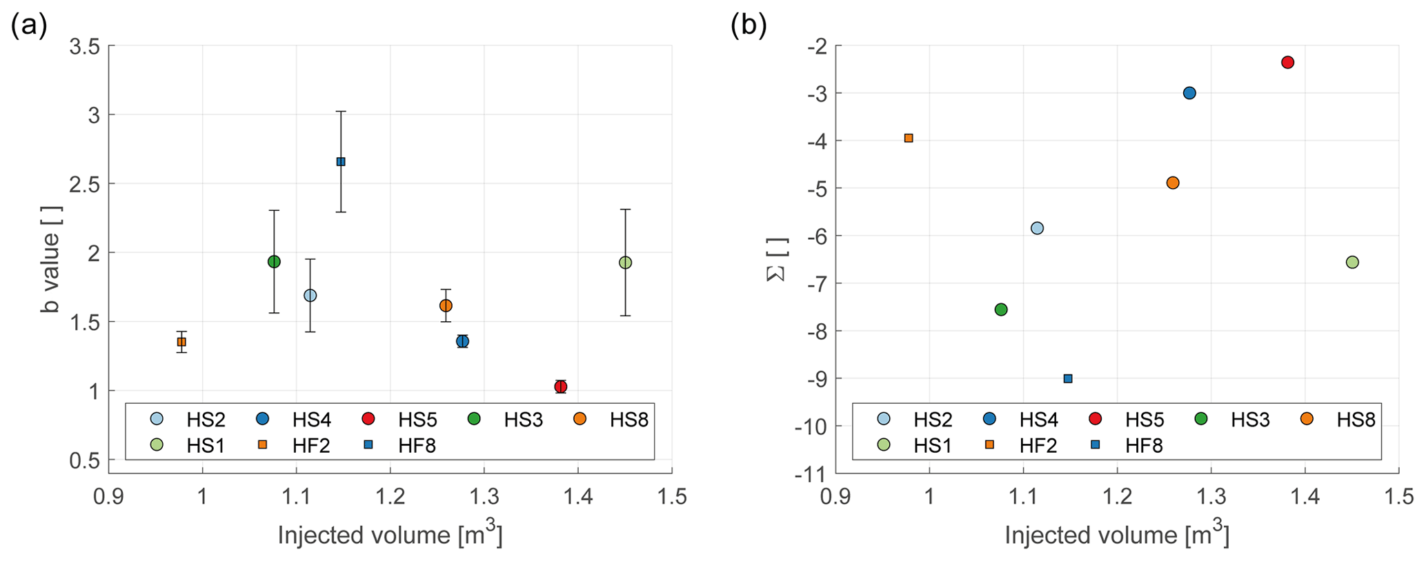
Figure 11(a) b values along with uncertainties plotted against seismically activated area and (b) seismogenic indices plotted against seismically activated area from experiments for which the b values, seismogenic indices, and areas could be estimated.
4.5 Seismic injection efficiency and ratio of seismic/aseismic deformation
In the following, we estimate the seismic moment release (referred to as M0 seismic) and compare it with a quantity termed hydraulic moment release (M0 hydraulic) as well as with the total moment release (M0 total) by stimulation experiment (Fig. 12).
The lower-bound estimate of M0 seismic during each injection experiment was determined by adding up the seismic moment of each located seismic event during the respective injection experiment. In order to estimate the experimental specific upper bound of the seismic moment release, the Gutenberg–Richter a and b values, determined in Sect. 4.3, were used to extrapolate the seismicity rates down to a magnitude of −9. Such small magnitudes were observed on the laboratory scale by Selvadurai (2019). Also McLaskey and Lockner (2014) and Yoshimitsu et al. (2014) observed very small magnitudes (i.e., M−7) and self-similarity down to these magnitudes. In situ, Goodfellow and Young (2014) observed magnitudes down to −7.5. For an average estimate of the seismic moment release, magnitudes down to a minimum magnitude of −6 were included (symbols in Fig. 12b). A high range of possible seismic moment release was observed for injection experiments with high b values (i.e., HS1, HS3, HF8), because the small-magnitude seismic events strongly contribute to the cumulative seismic moment release. Assuming the average estimate scenario and cumulating the moment release of all possible seismic events per injection experiment into a single earthquake would have induced a moment magnitude Mw in the range of −3 to −1. Assuming a stress drop of 1 or 0.1 MPa, respectively, and a source model by Brune (1970), this would correspond to a source radius of 0.3–2.2 m/0.6–4.8 m and a ruptured area of 0.26–15.5 m2/0.28–18 m2).
The equivalent hydraulic moment (M0 hydraulic) was calculated from the determined hydraulic injection energy. The hydraulic injection energy was estimated using , where p is the injection pressure, and Q is the injection flow rate, which are both integrated over the entire injection time. The pumped hydraulic energy is then converted to an equivalent seismic moment using (Aki and Richards, 2002; De Barros et al., 2019), where μ is the shear modulus, chosen to be 30 GPa, and Δσ represents the static stress drop assumed to be between 1 and 0.1 MPa. The average estimate represents the equivalent seismic moment averaging the aforementioned stress drop range (Fig. 12c).
The total moment (M0 total) released by stimulation can be estimated from borehole dislocations in the injection interval that was determined from acoustic televiewer (ATV) measurements before and after each injection experiment (i.e., for injection experiment HS2: 0.95 mm; for HS4: 0.95 mm; for HS3: 1.25 mm; for HS8: 0.45 mm; and for HS1: 0.75 mm; see Krietsch et al., 2020). Note that this is only possible for HS experiments, since in the HF experiments no fault dislocations were observed (Dutler et al., 2019). For the estimate of the seismic moment from the measured displacements at the injection interval, we used M0=μAD, where μ is the shear modulus, again chosen to be 30 GPa, A is the seismically activated area determined in Sect. 4.2, and D is the average slip on the area of rupture. For a lower-bound estimate, we assume that an average slip over the entire lower-bound seismically activated area (i.e., the concave hull area; see Sect. 4.2) is 10 % of the observed slip at the injection interval. For the upper-bound estimate, we assume that the average slip across the entire upper bound seismically activated area (i.e., the convex hull area estimate) corresponds to 50 % of the observed slip at injection intervals. Twenty-five percent of the observed slip and 50 % of the estimated seismically activated area were used for the average estimate of total moment release (symbols in Fig. 12d).
To estimate seismic injection efficiencies (i.e., the ratio between seismic moment released to equivalent hydraulic moment, Fig. 12e) and the ratio between seismic and total deformation (Fig. 12f), the average estimates of the equivalent hydraulic and total moment were used. The cumulative seismic moment release was varied according to the minimum magnitude at which seismicity rates were extrapolated. When integrating to a minimum magnitude of −6, seismic injection efficiencies lie in the range of (HS3) and (HF8); injection experiment HS4 showed a high value of with minor changes as the integration magnitude decreased, due to the low b value (i.e., due to the small contribution of small-magnitude events to the cumulative seismic moment). Seismic injection efficiencies (excluding experiment HF8) tended to converge to a value in the range of (HF2) and (HS1) when integrating to a minimum magnitude of −9.
The ratio between seismic and total moment release (Fig. 12f), considering events with magnitudes down to −6, ranged from (HS3) to (HS4). Integrating the seismic moment to a minimum magnitude of −9 leads to a convergence of the ratio between seismic and total deformation to values of (HS3) to (HS1).
We emphasize that the cumulative seismic moment, the equivalent hydraulic moment, and the equivalent total moment from dislocation observations are prone to a high level of uncertainty. Thus, uncertainties in the seismic injection efficiencies and the ratio between seismic and total moment give only crude estimates with uncertainties that possibly exceed 1 order of magnitude.
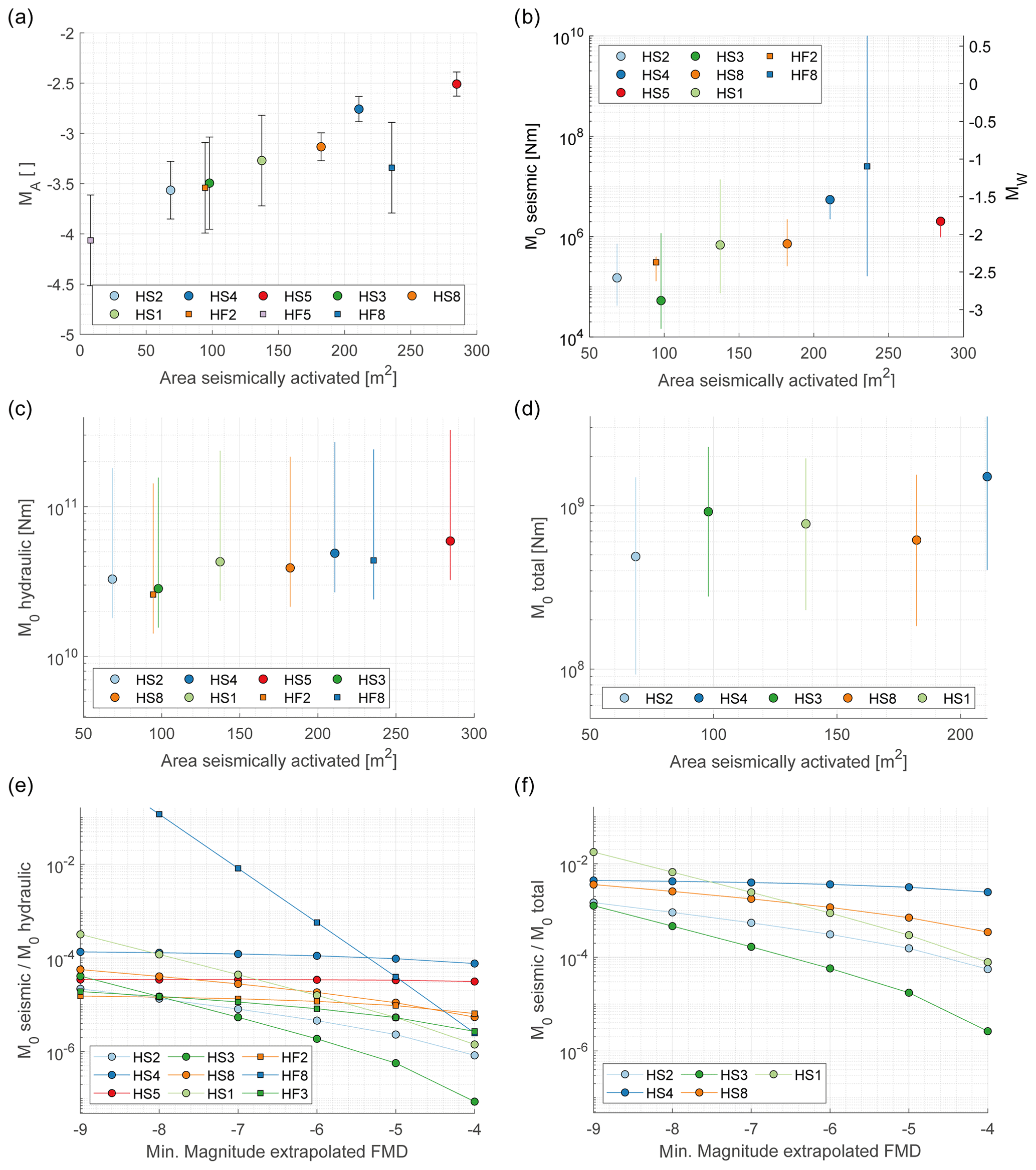
Figure 12(a) Maximum observed magnitudes (error bars represent the standard deviation of all magnitude estimates of the respective event) with respect to seismically activated area (the estimated seismically activated area represents the mean between the upper and lower bound of the area estimate of Sect. 4.2). (b) Estimated radiated seismic moment from extrapolated Gutenberg–Richter parameter (upper-bound and average estimate) and located seismic events (lower bound) along with the equivalent moment magnitude. (c) Equivalent hydraulic moment estimated from injection parameter (i.e., flow rate, injection pressure). (d) Equivalent moment estimate from acoustic televiewer displacement measurements at the injection interval. (e) Seismic injection efficiency against the magnitude level used for seismic moment extrapolation. (f) Ratio between seismic moment and equivalent seismic moment estimated from displacement measurements against the magnitude level used for seismic moment extrapolation.
The hydraulic stimulation experiments performed at the Grimsel Test Site aimed to investigate the influence of different geological settings (i.e., pre-existing fractures with variable orientation and architecture, HS, and intact rock, HF) on high-pressure fluid injection in terms of induced seismicity, permeability increase, pressure propagation, and rock deformation. Short borehole intervals of 1–2 m length were stimulated with standardized injection protocols – one each for the HS and HF experiments – and a total injected volume of about 1 m3. The injection protocol differed for HS and HF because, during HF experiments, the formation breakdown pressure of the rock had to be overcome for fracture initiation, while shearing during HS experiments can be initiated at pressures below the minimum principle stress. Thus, the HF experiments required higher injection rates and pressures than the HS experiments. It is also important to mention that the HF experiments were conducted in the same rock volume after the HS experiments were completed, which may have already altered the stress conditions in the rock mass. We argue that despite these differences between HS and HF experiments, comparing the process characteristics of all injection experiments is justified.
A high-quality catalog of earthquakes in a magnitude range MA of −2.5 to −6.2 was produced by the 11 injection experiments. The majority of located seismic events occurred during active pumping phases. A steady rate of located events throughout the experiments as well as an increased seismic response (i.e., a comparable low b value and a high seismogenic index) was observed for injections targeting the highly conductive brittle–ductile shear zones S3. Experiments targeting the more ductile shear zones S1 exhibit more intense seismicity at the beginning of the experiment and lower overall seismic responses compared to the injection experiments targeting S3 shear zones. Seismic responses of HF experiments do not systematically differ from seismic responses of HS experiments, even though during HF experiments less seismic events could be located. Seismicity from HS experiments often align with the targeted structures with some exemptions. Spatial distribution of seismicity for both HS and HF experiments can usually be approximated by a single plane. However, in some cases the spatial distribution is more complex with seismicity clustering in small subparallel seismicity clouds. The propagation direction of seismicity can change in the course of an experiment. Scoping calculations indicate that deformation may be to a large extent aseismic. The following subsections elaborate on specific questions in a broader context. The final section provides implications drawn from the performed experiments for a safe EGS reservoir development and the management of induced seismicity.
5.1 A highly variable seismic response and the role of geology
Remarkable is the large variability in the seismic responses between experiments conducted within less than a 25 m borehole length, which is expressed in the wide range of seismogenic indices (−9 to −2) and b values (1 to 2.7) (Fig. 11). The number of detected and located events during a stimulation depends on the detection ability of the sensor network, which is primarily a function of the distance (Mignan et al., 2011). However, even at a homogeneous completeness level of −4.02, the seismic response varies widely (Fig. 5c, d). Such variability is comparable to the variability between cases worldwide, involving both projects with predominant HF stimulation in the shale gas context and HS for geothermal exploitation (Fig. 13c, Dinske and Shapiro, 2013; Mignan et al., 2017). While Dinske and Shapiro (2013) suggest that there is a large difference in the seismic response during HF-dominated stimulations in shale gas projects and HS-dominated stimulations in geothermal applications, a systematic difference between the HS and HF experiments performed in crystalline rock was not discernible here. Also, the use of the shear-thinning xanthan–salt–water mixture during the HF experiments did not have an observable effect on the seismic response. The fact that the HF experiments were conducted in a rock mass where previous HS experiments could potentially have initiated some stress relaxation may explain the tendency for fewer events during the HF experiments. Experiment HF6, which can be interpreted as continuation of the HS1 experiment, induced only a few seismic events because the zone was stimulated twice. In contrast, the dispersed character of seismic events in the HF3 experiment may be explained by the interaction of new fractures with the surrounding faults S1.0, S3.1, and S3.2. We conclude that in our experiments HS and HF are similarly seismogenic, because HF strongly interacts with the pre-existing fracture network leading to similar seismic responses as the injections directly into pre-existing fractures.
While differences in the seismic response between HF and HS were not evident, the geological setting seems important for the substantial differences seen in the seismic response in terms of magnitude distributions as well as in terms of orientation and propagation of seismicity. We observed that experiments performed directly on or in the vicinity of the highly fractured brittle–ductile S3 shear zones (Fig. 13a, i.e., experiments HS5, HS4, and HS8 and HF3, respectively) are characterized by an enhanced seismic response. This observation is in agreement with the hypothesis gained from larger-scale stimulations, which states that well-developed brittle fault zones (i.e., connecting fractures that form larger features) lead to a comparatively high seismic moment release in response to high-pressure fluid injection (McClure and Horne, 2014b; De Barros et al., 2016). An exception is experiment HF2, which shows an increased seismic response with possibly no influence from S3 structures. Injection experiment HF2 was performed between the ductile shear zones S1.1 and S1.2, north of shear zone S3. At this location the reactivated structure (i.e., Cluster 1 and Cluster 2 of HF2; see also Fig. 7) may support an increased amount of shear stress, which led to an increased seismic response.
Not only do the seismic responses (i.e., b value and the seismogenic indices) indicate a strong geological influence but also the seismicity detection rate in relation to injected volume (Fig. 5) shows a different seismic footprint for the two shear zone types. For the injection experiments on the ductile shear zones (S1) more than 50 % of all detections are made during the injection of the initial 100 L of fluid. In contrast, the S3 shear zones experienced a gradual increase in detections with injected fluid volume (Fig. 5a).
The spatial distribution and propagation also appear to be affected by the geology. A concentric growth of seismicity clouds was rarely observed, indicating that the spatial fracture zone heterogeneity had a substantial impact. Seismicity clouds of experiments on ductile shear zones S1 show changing propagation directions and a planar character. Comparing the two S3 stimulations (HS4 and HS5), distinct differences in seismicity patterns were observed, even for stimulations within 3 m from each other in similar geological structures. During HS5, propagation directions changed along an extended seismicity cloud (of 16 m diameter) with a clustered character and regions of increased seismic event density. During the HS4 experiment the seismicity was mostly limited to patches/clusters within a 9 m radius from the injection interval but with a complex 3D and nonplanar architecture (Figs. 6, 8).
Beside their tendency of being very seismogenic, the highly fractured S3 shear zones stand out as being the most hydraulically conductive structures in the experimental volume compared to the less conductive S1 shear zones (see injectivities of HS4 and HS5 intervals in Fig. 13b). Injectivities at these intervals only increased marginally during stimulation. On the contrary, injectivities for the S1 stimulation experiments on the ductile shear zones and in the intact intervals increased by 2–3 orders of magnitude. Again, these observations agree with cases in the literature, for which the most permeable fractures were also found to be the most critically stressed and thus the most seismogenic zones (e.g., Barton et al., 1988; Barton et al., 1995; Barton and Zoback, 1998; Evans et al., 2005a; Davatzes and Hickman, 2010; Baisch et al., 2015; Hirschberg et al., 2015). It is also noteworthy that the injectivities for all experiments performed at the brittle–ductile shear zones, the ductile shear zones, and in the intact intervals end up having the same order of magnitude (Fig. 13b). While initial injectivities are highly dependent on the local geology, final injectivities are very similar (as are transmissivities; Brixel et al., 2020).
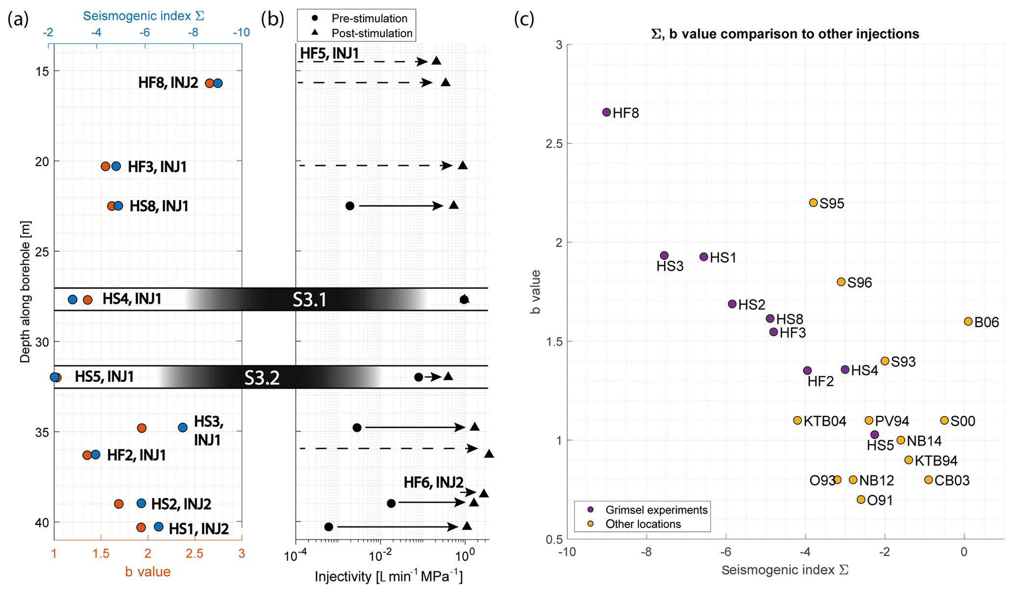
Figure 13(a) Seismic responses (seismogenic indices, b values) along with (b) pre- and post-injectivity values of experiments along the depth of the injection boreholes. Location of S3 shear zones and experiment HS4 and HS5 therein are highlighted. Injectivity values of experiment HF5 and HF6 for which the number of located seismic events renders a determination of b value and seismogenic index impossible, are also included. (b) b values and seismogenic indices of various high-pressure fluid injections at different sites (source seismogenic indices and b values from other locations: Dinske and Shapiro, 2013; Shapiro et al., 2013; and Mignan et al., 2017).
With the aforementioned observations in mind, it is possible to imagine what would have happened if a large open-hole stimulation would have been conducted in INJ1 and INJ2, as it was done in most of the previous EGS projects (e.g., Basel, Häring et al., 2008; Soultz, Evans et al., 2005b), instead of several stimulations at selected short intervals. Because of their high transmissivity, flow would have preferentially entered the shear zones S3.1 and S3.2 leading to induced seismicity, mostly dominated by the seismogenic properties of these structures. The result would have been a very limited transmissivity increase together with a strong seismic response. Thus, for larger-scale EGS stimulations, it appears quite promising to selectively stimulate multiple short borehole intervals with comparatively small fluid volumes (i.e., zonal isolation, Meier et al., 2015), during which the transmissivity of low-transmissive structures would be strongly enhanced, while stimulations in intervals at seismogenic fault zones should be avoided if possible. Of course, hydraulic stimulation of short intervals could also be combined with alternative injection schemes (such as described by Zang et al., 2017). However, the pronounced influence of geology on the aforementioned stimulation parameters in our experiments may imply that the impact of alternative injection strategies on induced seismicity (such as those discussed and proposed in the literature by McClure and Horne, 2011; Zimmermann et al., 2014; McClure et al., 2016; and Zang et al., 2018) is limited, since their effects are unlikely to emerge above the strong variability of orders of magnitudes imposed by the geological conditions.
5.2 Impact of the stress field
Compared to the observed main orientation of the S1 (NE–SW) and the S3 (E–W) shear zones in the tunnels surrounding the experimental volume, the orientation of individual fractures within the S1 and S3 fault zones do show a similar WSW–ENE orientation. Also, the orientation of fractures found in the host rock are predominantly WSW–ENE in orientation with some random joint orientations. We combine the orientation of these pre-existing fractures with the slip tendencies inferred from the stress conditions measured 30 m south of shear zone S3.1 (i.e., the unperturbed stress state) and the stress conditions measured in borehole SBH4 (Fig. 2) in the vicinity of shear zone S3.1 (i.e., the perturbed stress state). It can be seen that there is an increased susceptibility for the S1 and S3 structures to slip (see also Krietsch et al., 2018a) when considering the perturbed stress state (Fig. 14a, b).
By including both the inferred orientation of the seismicity clouds or their clusters resulting from the injection experiments performed on the shear zones (i.e., the HS experiments) and the stress field, the combined influence of geology and stress field becomes evident. The predominant orientation of seismicity clouds is E–W, in agreement with the orientation of pre-existing fractures. Surprisingly, the predominant orientation also holds for the S1 stimulation experiments, even though the main orientation of the S1 shear-zones is NE–SW. Only the seismicity cloud of injection experiment HS1 is oriented in the main S1 direction. However, the orientation of seismicity in the E–W direction, also for S1 experiments, is not surprising when considering the fracture inventory of the experimental volume and the overlapping pole points of S1 and S3 structures, as well as the increased fracture density with the same orientation (Fig. 14a–d).
Hydraulic fractures in a strict sense, meaning fractures which form in intact rock, perpendicular to the minimum principal stress, at injection pressures higher than the minimum principal stress, are conceivable for the initiated fractures in experiment HF5 and the initial fracture (Cluster 1) of experiment HF2, oriented perpendicular to the minimum principal stress of the perturbed stress state where directional geological features are sparse. Cluster 2 of experiment HF2 formed at a later time compared to Cluster 1; it possibly formed because of the leak-off of fluids through Cluster 1 to the formation. The associated reduction in pore pressure through Cluster 1 may suggest a geology-dominated E–W orientation of the seismicity cloud of Cluster 2.
The new fracture created during experiment HS4 (Cluster 3) orients in a direction perpendicular to the minimum principal stress of the perturbed stress field (Villiger et al., 2019). We suggest that this fracture opens in connection to shear dislocation along shear zone S3.1 (Jung, 2013) induced during the HS4 injection.
In conclusion, the perturbed stress field – measured closer to the target rock volume than the unperturbed stress field – explains most of the observed seismicity cloud orientations well. HFs growing through intact rock tend to form normal to the minimum principal stress, while the other seismicity clouds are mostly guided by the predominant set of geological features that have comparably high slip tendency. However, it is likely that local stress variations may locally lead to a combination of opening mode deformation (i.e., mode I opening) and shear dislocation (mode II, mode III). Also, HFs show a strong tendency to connect with the pre-existing fracture network, which might explain why the seismic response during HF experiments is similar to the one during HS experiments.
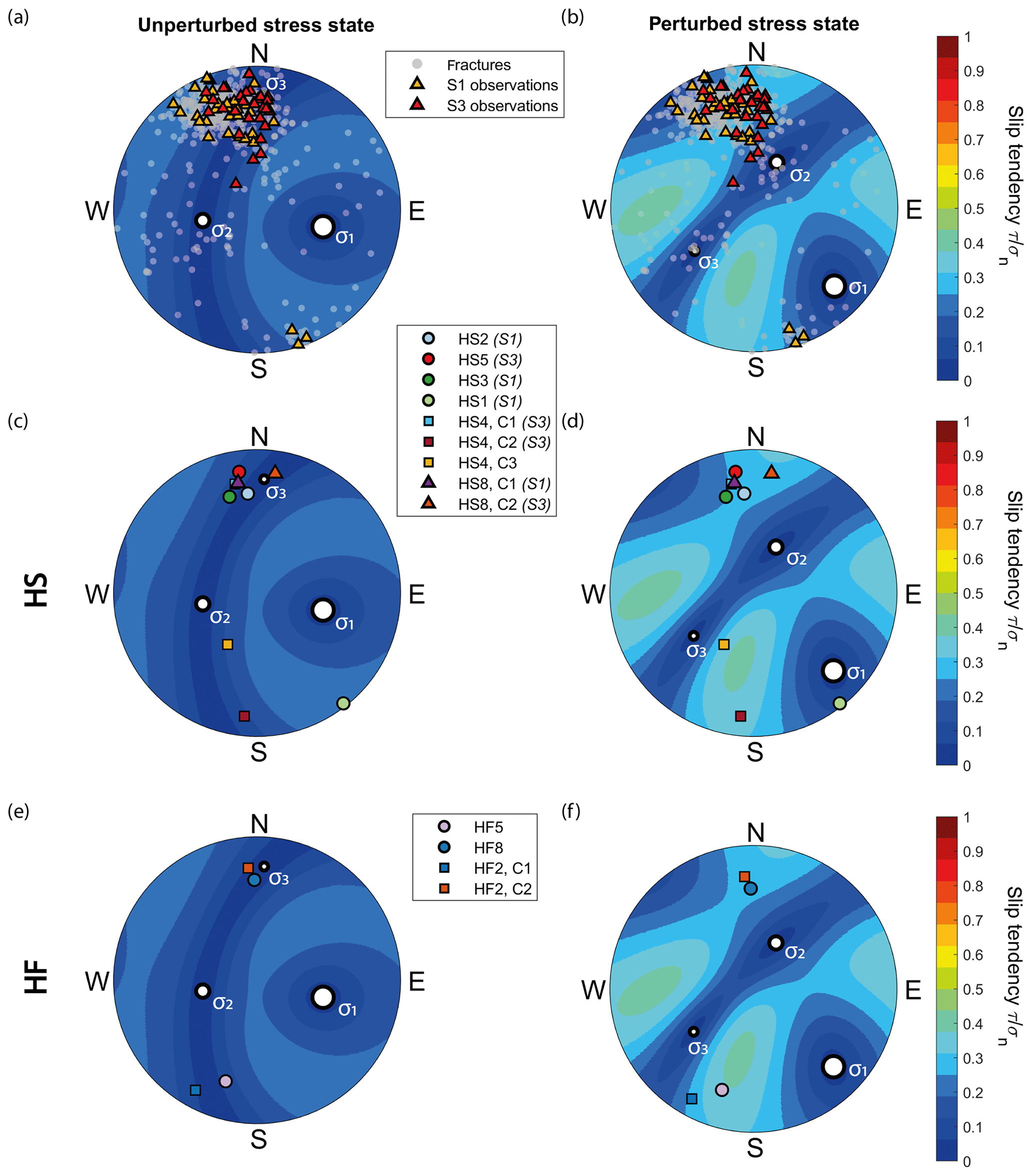
Figure 14Principal stress directions of the unperturbed (σ1=13.1 MPa, 104∘ dip direction/39∘ dip; σ2=9.2 MPa, ; and σ3=8.7 MPa, ) and perturbed stress state (σ1=13.1 MPa, 134∘ dip direction/14∘ dip; σ2=8.2 MPa, ; and σ3=6.5 MPa, ) along with slip tendencies determined from the respective stress state in lower-hemisphere stereographic plots, along with (a, b) the fracture inventory from borehole observations, (c, d) pole points of seismicity cloud orientations of HS experiments, their targeted structures and (e, f) orientation of seismicity clouds of HF stimulation experiments.
5.3 Aseismic deformation
Our experiments indicate that deformation in HS experiments (for which a displacement was measured at the injection interval) is to a large extent aseismic (i.e., < 2 % seismic). We also observed the tendency for the amount of aseismic deformation to be larger for experiments targeting the S1 structures (Fig. 12f). These overall values agree with values determined from hydraulic reactivation of a fault zone in limestone on a decameter scale, where 0.1 % to 3.9 % of shear deformation was estimated to be seismic (Duboeuf et al., 2017). Similar studies in shale materials report that less than 0.1 % of deformation is seismic (De Barros et al., 2016). An increased value of 4 % to 8 % for released seismic energy was reported for hydraulic fracturing experiments on granite samples at the laboratory scale (Goodfellow et al., 2015). Also, at the field scale, a large amount of aseismic deformation is suspected due to the observed slip dislocation of up to 4 cm on an acoustic televiewer log of an injection interval in granite at Soultz-sous-Forêts, which is much larger than the slip motion associated with the recorded seismic events (Cornet et al., 1997).
Seismic risk management is a key requirement for the sustainable development of deep geo-energy, such as EGS (Grigoli et al., 2017; Trutnevyte and Wiemer, 2017; Lee et al., 2019). In the following, we propose potential implications for induced seismic risk management from our GTS experiments:
Anticipate variability. Despite comparable injection strategies and injection intervals being located within a few tens of meters, the seismic response in terms of productivity and size distribution is surprisingly variable (e.g., Fig. 10). While an explanation for such variability may be found in retrospect, forecasting the expected seismic hazard during future injections at the GTS could be affected by large uncertainties. Thus, large uncertainties in seismic hazard forecasts for less well-known, well-characterized, and well-monitored sites have to be anticipated. However, at the same time, the seismic response during stimulations is often surprisingly easily predictable via injected fluid volume once an estimate of the site-specific, time-invariable seismogenic index is available (Mignan et al., 2017). Possibly, the variability in the seismic response, as we observed it at the GTS, would be unified, once multiple faults in a larger region are stimulated. However, our observations suggest that the seismic response would not be an average response but rather correspond to the seismic response of the most seismogenic structures in the stimulated volume.
Update induced seismic hazard forecasting. Since a priori estimates of the seismic response of a stimulation are difficult, improved forecasts with more confidence in the expected seismicity may be done after initial testing. Figure 5 illustrates that, based on the initial 200 L of injected volume, it is possible to roughly forecast the overall productivity. While these forecasting strategies will need to be formally tested (e.g., following the approaches of Király-Proag et al., 2016, 2017; Broccardo et al., 2017), it suggests that the strategies used for adaptive traffic light systems (e.g., Grigoli et al., 2017; Mignan et al., 2017) are required and can be successful. This is also in line with the recommendation of the Pohang investigation (Lee et al., 2019).
Injection strategies. Our study shows the pronounced influence of geology on induced seismicity during high-pressure fluid injection. It may be possible that alternative injection schemes could have a similar pronounced impact on the seismic response, but this has yet to be proven. Our results clearly suggest that great care is necessary when evaluating different injection schemes, as even within the same geological unit, the rock architecture has a pronounced influence, which raises the questions of whether it is possible to find two or more sites within an in situ experiment that are similar enough to neglect the influence of geology and concentrate solely on the influence of different injection protocols.
Selective stimulation (zonal isolation). The Grimsel results recommend the concept of zonal isolation (i.e., the selective stimulation of short borehole sections). In an open hole stimulation, most injected fluid may have only entered the most transmissive shear zones and increased their transmissivity marginally but at the cost of an increased seismic response. From our experiment, we conclude that not only a single pre-stimulation test per site but also a pre-stimulation in each isolated zone should be performed. Such pre-stimulations with small fluid volumes would not only allow estimation of the initial hydraulic properties but also provide a learning phase for seismicity forecasting models. Furthermore, they identify not only structures with an increased seismic response but also less seismogenic structures that have a larger propensity for aseismic slip. As a consequence, one should be able to skip and seal isolated zones where an increased seismic response or the chance of hydraulic short-circuits is anticipated and focus stimulation in less seismogenic zones. However, how representative a pre-stimulation in an isolated zone is for the further course of stimulation and the feasibility of zonal isolation techniques in the context of EGS have yet to be tested. The zonal isolation technique and the ability to seal isolated zones would certainly offer more flexibility and opportunities to intervene in case of elevated seismicity levels.
The Grimsel ISC Experiment Description is available at https://doi.org/10.3929/ethz-b-000310581 (Doetsch et al., 2018a) The seismic dataset, as well as hydraulic data of the Grimsel ISC hydraulic shearing and hydraulic fracturing experiments, can be found at https://doi.org/10.3929/ethz-b-000280357 (Villiger et al., 2018).
The supplement related to this article is available online at: https://doi.org/10.5194/se-11-627-2020-supplement.
The monitoring setup was designed by VSG, JD, LV, HK, MJ, and FA. The injection protocol for the HS experiments was designed by VSG, JD, MJ, and FA. The injection protocol for the HF experiments was designed by NOD and BV. VSG, JD, LV, HK, MJ, FA, NOD, and BV were part of the team performing the HS and HF experiments during the ISC project; FA was the project administrator. The formal analysis, data curation, and data visualization, including writing the original draft, were done by LV with the help of VSG and SW. The review and editing of the paper were done by all the authors.
The authors declare that they have no conflict of interest.
This study is part of the In-situ Stimulation and Circulation (ISC) project established by the Swiss Competence Center for Energy Research - Supply of Electricity (SCCER-SoE) with the support of Innosuisse. Funding for the ISC project was provided by the ETH Foundation with grants from Shell and EWZ and by the Swiss Federal Office of Energy through a P&D grant. The Grimsel Test Site is operated by Nagra, the National Cooperative for the Disposal of Radioactive Waste. We are indebted to Nagra for hosting the ISC project in their facility and to the Nagra technical staff for on-site support.
This research has been supported by the Swiss Federal Institute of Technology Zurich (grant no. ETH-35 16-1, Linus Villiger) and the Swiss National Foundation (grant nos. 200021_165677 (Nathan Dutler), 200021_169178 (Hannes Krietsch)).
This paper was edited by Michal Malinowski and reviewed by two anonymous referees.
Aki, K. and Richards, P. G.: Quantitative seismology, 2nd ed., edited by: Ellis, J., Sausalito, CA, University Science Books, 2002.
Amann, F., Gischig, V., Evans, K., Doetsch, J., Jalali, R., Valley, B., Krietsch, H., Dutler, N., Villiger, L., Brixel, B., Klepikova, M., Kittilä, A., Madonna, C., Wiemer, S., Saar, M. O., Loew, S., Driesner, T., Maurer, H., and Giardini, D.: The seismo-hydromechanical behavior during deep geothermal reservoir stimulations: open questions tackled in a decameter-scale in situ stimulation experiment, Solid Earth, 9, 115–137, https://doi.org/10.5194/se-9-115-2018, 2018.
Atkinson, G. M., Eaton, D. W., Ghofrani, H., Walker, D., Cheadle, B., Schultz, R., Shcherbakov, R., Tiampo, K., Gu, J., and Harrington, R. M.: Hydraulic fracturing and seismicity in the Western Canada Sedimentary Basin, Seismol. Res. Lett., 87, 631–647, 2016.
Baisch, S., Rothert, E., Stang, H., Vörös, R., Koch, C., and McMahon, A.: Continued geothermal reservoir stimulation experiments in the Cooper Basin (Australia), B. Seismol. Soc. Am., 105, 198–209, 2015.
Barbosa, N., Carspari, E., Rubino, G., Greenwood, A., Ludovic, B., and Klaus, H.: Estimation of fracture compliance from attenuation and velocity analysis of full-waveform sonic log data, J. Geophys. Res.-Sol. Ea., 124, 2738–2761, 2019.
Barton, C. A. and Zoback, M. D.: Earth stress, rock fracture and wellbore failure – Wellbore imaging technologies applied to reservoir geomechanics and environmental engineering, Tokyo, Japan, December, 49–56, 1998.
Barton, C. A., Zoback, M. D., and Burns, K. L.: In-situ stress orientation and magnitude at the Fenton Geothermal Site, New Mexico, determined from wellbore breakouts, Geophys. Res. Lett., 15, 467–470, 1988.
Barton, C. A., Zoback, M. D., and Moos, D.: Fluid flow along potentially active faults in crystalline rock, Geology, 23, 683–686, 1995.
Boatwright, J.: Detailed spectral analysis of two small New York State earthquakes, B. Seismol. Soc. Am., 68, 1117–1131, 1978.
Bohnhoff, M., Dresen, G., Ellsworth, W. L., and Ito, H.: Passive seismic monitoring of natural and induced earthquakes: case studies, future directions and socio-economic relevance, in: New Frontiers in Integrated Solid Earth Sciences, Springer, 261–285, 2009.
Brixel, B., Klepikova, M., Jalali, M. R., Lei, Q., Roques, C., Krietsch, H., and Loew, S.: Tracking fluid flow in shallow crustal fault zones: 1. Insights from single‐hole permeability estimates, J. Geophys. Res.-Sol. Ea., 125, https://doi.org/10.1029/2019JB018200, 2020.
Broccardo, M., Mignan, A., Wiemer, S., Stojadinovic, B., and Giardini, D.: Hierarchical Bayesian Modeling of Fluid-Induced Seismicity, Geophys. Res. Lett., 44, 11357–311367, 2017.
Brown, D. W., Duchane, D. V., Heiken, G., and Hriscu, V. T.: Mining the earth's heat: hot dry rock geothermal energy, Springer Science & Business Media, Berlin, Heidelberg, 2012.
Brune, J. N.: Tectonic stress and the spectra of seismic shear waves from earthquakes, J. Geophys. Res., 75, 4997–5009, 1970.
Catalli, F., Rinaldi, A. P., Gischig, V., Nespoli, M., and Wiemer, S.: The importance of earthquake interactions for injection induced seismicity: Retrospective modeling of the Basel Enhanced Geothermal System, Geophys. Res. Lett., 43, 4992–4999, 2016.
Cornet, F., Helm, J., Poitrenaud, H., and Etchecopar, A.: Seismic and aseismic slips induced by large-scale fluid injections, in: Seismicity associated with mines, reservoirs and fluid injections, Springer, Birkhäuser, Basel, 563–583, 1997.
Davatzes, N. C. and Hickman, S. H.: Stress, fracture, and fluid-flow analysis using acoustic and electrical image logs in hot fractured granites of the Coso geothermal field, California, USA, 2010.
De Barros, L., Daniel, G., Guglielmi, Y., Rivet, D., Caron, H., Payre, X., Bergery, G., Henry, P., Castilla, R., and Dick, P.: Fault structure, stress, or pressure control of the seismicity in shale? Insights from a controlled experiment of fluid-induced fault reactivation, J. Geophys. Res.-Sol. Ea., 121, 4506–4522, 2016.
De Barros, L., Cappa, F., Guglielmi, Y., Duboeuf, L., and Grasso, J.-R.: Energy of injection-induced seismicity predicted from in-situ experiments, Sci. Rep.-UK, 9, 1–11, 2019.
Dinske, C.: Interpretation of fluid-induced seismicity at geothermal and hydrocarbon reservoirs of Basel and Cotton Valley, PhD thesis, Freie Universität Berlin, Berlin, 2011.
Dinske, C. and Shapiro, S. A.: Seismotectonic state of reservoirs inferred from magnitude distributions of fluid-induced seismicity, J. Seismol., 17, 13–25, 2013.
Doetsch, J., Gischig, V., Krietsch, H., Villiger, L., Amann, F., Dutler, N., Jalali, M., Brixel, B., Roques, C., Giertzuch, P., Kittilä, A., and Hochreutener, R.: Grimsel ISC Experimental Description, https://doi.org/10.3929/ethz-b-000310581, 2018a.
Doetsch, J., Gischig, V., Villiger, L., Krietsch, H., Nejati, M., Amann, F., Jalali, M., Madonna, C., Maurer, H., and Wiemer, S.: Subsurface Fluid Pressure and Rock Deformation Monitoring using Seismic Velocity Observations, Geophys. Res. Lett., 45, 10–389, 2018b.
Dresen, G., Renner, J., Bohnhoff, M., Konietzki, H., Kwiatek, G., Plenkers, K., Klee, G., and Backers, T.: STIMTEC – a mine-back experiment in the Reiche Zeche underground laboratory, EGU General Assembly 2019, Vienna, 2019.
Duboeuf, L., De Barros, L., Cappa, F., Guglielmi, Y., Deschamps, A., and Seguy, S.: Aseismic motions drive a sparse seismicity during fluid injections into a fractured zone in a carbonate reservoir, J. Geophys. Res.-Sol. Ea., 122, 8285–8304, 2017.
Dutler, N., Valley, B., Gischig, V., Villiger, L., Krietsch, H., Doetsch, J., Brixel, B., Jalali, M., and Amann, F.: Hydraulic fracture propagation in a heterogeneous stress field in a crystalline rock mass, Solid Earth, 10, 1877–1904, https://doi.org/10.5194/se-10-1877-2019, 2019.
Economides, M. J. and Nolte, K. G.: Reservoir stimulation, Prentice Hall Englewood Cliffs, NJ, 1989.
Eisenblätter, J. and Spies, T.: Ein Magnitudenmaß für Schallemissionsanalyse und Mikroakustik, Deutsche Gesellschaft für zerstörungsfreie Prüfung, 12, Kolloquium Schallemission, 29–41, 2000.
Ellsworth, W. L.: Injection-induced earthquakes, Science, 341, 1225942, https://doi.org/10.1126/science.1225942, 2013.
Evans, K., Moriya, H., Niitsuma, H., Jones, R., Phillips, W., Genter, A., Sausse, J., Jung, R., and Baria, R.: Microseismicity and permeability enhancement of hydrogeologic structures during massive fluid injections into granite at 3 km depth at the Soultz HDR site, Geophys. J. Int., 160, 388–412, 2005a.
Evans, K. F., Genter, A., and Sausse, J.: Permeability creation and damage due to massive fluid injections into granite at 3.5 km at Soultz: 1. Borehole observations, J. Geophys. Res.-Sol. Ea., 110, B04203, https://doi.org/10.1029/2004JB003168, 2005b.
Evans, K. F., Zappone, A., Kraft, T., Deichmann, N., and Moia, F.: A survey of the induced seismic responses to fluid injection in geothermal and CO2 reservoirs in Europe, Geothermics, 41, 30–54, 2012.
Fehler, M. C.: Stress control of seismicity patterns observed during hydraulic fracturing experiments at the Fenton Hill hot dry rock geothermal energy site, New Mexico, International Journal of Rock Mechanics and Mining Sciences & Geomechanics Abstracts, 211–219, 1989.
Gischig, V. S.: Rupture propagation behavior and the largest possible earthquake induced by fluid injection into deep reservoirs, Geophys. Res. Lett., 42, 7420–7428, 2015.
Gischig, V. S., Doetsch, J., Maurer, H., Krietsch, H., Amann, F., Evans, K. F., Nejati, M., Jalali, M., Valley, B., Obermann, A. C., Wiemer, S., and Giardini, D.: On the link between stress field and small-scale hydraulic fracture growth in anisotropic rock derived from microseismicity, Solid Earth, 9, 39–61, https://doi.org/10.5194/se-9-39-2018, 2018.
Goebel, T. and Brodsky, E. E.: The spatial footprint of injection wells in a global compilation of induced earthquake sequences, Science, 361, 899–904, 2018.
Goebel, T., Hosseini, S., Cappa, F., Hauksson, E., Ampuero, J., Aminzadeh, F., and Saleeby, J.: Wastewater disposal and earthquake swarm activity at the southern end of the Central Valley, California, Geophys. Res. Lett., 43, 1092–1099, 2016.
Goebel, T., Weingarten, M., Chen, X., Haffener, J., and Brodsky, E.: The 2016 Mw 5. 1 Fairview, Oklahoma earthquakes: Evidence for long-range poroelastic triggering at > 40 km from fluid disposal wells, Earth Planet. Sc. Lett., 472, 50–61, 2017.
Goodfellow, S. and Young, R.: A laboratory acoustic emission experiment under in situ conditions, Geophys. Res. Lett., 41, 3422–3430, 2014.
Goodfellow, S., Nasseri, M., Maxwell, S., and Young, R.: Hydraulic fracture energy budget: Insights from the laboratory, Geophys. Res. Lett., 42, 3179–3187, 2015.
Grigoli, F., Cesca, S., Priolo, E., Rinaldi, A. P., Clinton, J. F., Stabile, T. A., Dost, B., Fernandez, M. G., Wiemer, S., and Dahm, T.: Current challenges in monitoring, discrimination, and management of induced seismicity related to underground industrial activities: A European perspective, Rev. Geophys., 55, 310–340, 2017.
Grigoli, F., Cesca, S., Rinaldi, A., Manconi, A., López-Comino, J., Clinton, J., Westaway, R., Cauzzi, C., Dahm, T., and Wiemer, S.: The November 2017 Mw 5.5 Pohang earthquake: A possible case of induced seismicity in South Korea, Science, 360, 1003–1006, 2018.
Guglielmi, Y., Cappa, F., Avouac, J.-P., Henry, P., and Elsworth, D.: Seismicity triggered by fluid injection–induced aseismic slip, Science, 348, 1224–1226, 2015.
Haimson, B., and Fairhurst C.: In-situ stress determination at great depth by means of hydraulic fracturing. The 11th US symposium on rock mechanics (USRMS), American Rock Mechanics Association, 1969.
Häring, M. O., Schanz, U., Ladner, F., and Dyer, B. C.: Characterisation of the Basel 1 enhanced geothermal system, Geothermics, 37, 469–495, 2008.
Hirschberg, S., Wiemer, S., and Burgherr, P.: Energy from the Earth, Deep Geothermal as a Resource for the Future, chap. 3.2, 82–118, https://doi.org/10.3218/3655-8, 2015.
Holliger, K. and Bühnemann, J.: Attenuation of broad band (50–1500 Hz) seismic waves in granitic rocks near the Earth'surface, Geophys. Res. Lett., 23, 1981–1984, 1996.
Ingebritsen, S. E. and Manning, C.: Permeability of the continental crust: dynamic variations inferred from seismicity and metamorphism, Geofluids, 10, 193–205, 2010.
Jalali, M., Gischig, V., Doetsch, J., Näf, R., Krietsch, H., Klepikova, M., Amann, F., and Giardini, D.: Transmissivity Changes and Microseismicity Induced by Small Scale Hydraulic Fracturing Tests in Crystalline Rock, Geophys. Res. Lett., 45, 2265–2273, 2018.
Jung, R.: EGS – goodbye or back to the future, ISRM International Conference for Effective and Sustainable Hydraulic Fracturing, International Society for Rock Mechanics and Rock Engineering, 2013.
Kelkar, S., WoldeGabriel, G., and Rehfeldt, K.: Lessons learned from the pioneering hot dry rock project at Fenton Hill, USA, Geothermics, 63, 5–14, 2016.
Kim, K.-H., Ree, J.-H., Kim, Y., Kim, S., Kang, S. Y., and Seo, W.: Assessing whether the 2017 Mw 5.4 Pohang earthquake in South Korea was an induced event, Science, 360, 1007–1009, https://doi.org/10.1126/science.aat6081, 2018.
Király-Proag, E., Zechar, J. D., Gischig, V., Wiemer, S., Karvounis, D., and Doetsch, J.: Validating induced seismicity forecast models – Induced seismicity test bench, J. Geophys. Res.-Sol. Ea., 121, 6009–6029, 2016.
Király-Proag, E., Gischig, V., Zechar, J., and Wiemer, S.: Multicomponent ensemble models to forecast induced seismicity, Geophys. J. Int., 212, 476–490, 2017.
Kneafsey, T. J., Dobson, P., Blankenship, D., Morris, J., Knox, H., Schwering, P., White, M., Doe, T., Roggenthen, W., and Mattson, E.: An overview of the EGS Collab project: field validation of coupled process modeling of fracturing and fluid flow at the Sanford Underground Research Facility, Lead, SD, 43rd Workshop on Geothermal Reservoir Engineering, Stanford University, paper SGP-TR-213, available at: https://pangea.stanford.edu/ERE/pdf/IGAstandard/SGW/2018/Kneafsey.pdf (last access: 23 April 2020), 2018.
Krietsch, H., Doetsch, J., Dutler, N., Jalali, M., Gischig, V., Loew, S., and Amann, F.: Comprehensive geological dataset describing a crystalline rock mass for hydraulic stimulation experiments, Scientific Data, 5, 1–12, 2018a.
Krietsch, H., Gischig, V., Evans, K., Doetsch, J., Dutler, N. O., Valley, B., and Amann, F.: Stress Measurements for an In Situ Stimulation Experiment in Crystalline Rock: Integration of Induced Seismicity, Stress Relief and Hydraulic Methods, Rock Mech. Rock Eng., 52, 517–542, 2018b.
Krietsch, H., Villiger, L., Doetsch, J., Gischig, V., Evans, K., Brixel, B., Jalali, M., Loew, S., Giardini, D., and Amann, F.: Changing flow paths caused by simultaneous shearing and fracturing observed during hydraulic stimulation, Geophys. Res. Lett., 47, e2019GL086135, https://doi.org/10.1029/2019GL086135, 2019.
Krietsch, H., Gischig, V. S., Doetsch, J., Evans, K. F., Villiger, L., Jalali, M., Valley, B., Loew, S., and Amann, F.: Hydro-mechanical processes and their influence on the stimulation effected volume: Observations from a decameter-scale hydraulic stimulation project, Solid Earth Discuss., https://doi.org/10.5194/se-2019-204, in review, 2020.
Krischer, L., Smith, J., Lei, W., Lefebvre, M., Ruan, Y., de Andrade, E. S., Podhorszki, N., Bozdağ, E., and Tromp, J.: An Adaptable Seismic Data Format, Geophysical Supplements to the Monthly Notices of the Royal Astronomical Society, 207, 1003–1011, 2016.
Kwiatek, G., Plenkers, K., Dresen, G., and Group, J. R.: Source parameters of picoseismicity recorded at Mponeng deep gold mine, South Africa: Implications for scaling relations, B. Seismol. Soc. Am., 101, 2592–2608, 2011.
Kwiatek, G., Martínez Garzón, P., Plenkers, K., Leonhardt, M., Zang, A., von Specht, S., Dresen, G., and Bohnhoff, M.: Insights Into Complex Subdecimeter Fracturing Processes Occurring During a Water Injection Experiment at Depth in Äspö Hard Rock Laboratory, Sweden, J. Geophys. Res.-Sol. Ea., 123, 6616–6635, 2017.
Kwiatek, G., Saarno, T., Ader, T., Bluemle, F., Bohnhoff, M., Chendorain, M., Dresen, G., Heikkinen, P., Kukkonen, I., and Leary, P.: Controlling fluid-induced seismicity during a 6.1-km-deep geothermal stimulation in Finland, Science Advances, 5, eaav7224, https://doi.org/10.1126/sciadv.aav7224, 2019.
Lee, K., Yeo, I., Lee, J., Kang, T., Rhie, J., Sheen, D., Chang, C., Son, M., Cho, I., and Oh, S.: Summary report of the Korean Government Commission on relations between the 2017 Pohang earthquake and the EGS project, Geological Society of Korea and Korean Government Commission on the Cause of the Pohang Earthquake, S. 205, available at: http://www.gskorea.or.kr/custom/27/data/Summary_Report_on_Pohang_Earthquake_March_20_2019.pdf (last access: 24 April 2020), 2019.
Lee, K.-K., Ellsworth, W. L., Giardini, D., Townend, J., Ge, S., Shimamoto, T., Yeo, I.-W., Kang, T.-S., Rhie, J., and Sheen, D.-H.: Managing injection-induced seismic risks, Science, 364, 730–732, 2019.
Manthei, G., Eisenblätter, J., Spies, T., and Eilers, G.: Source parameters of acoustic emission events in salt rock, J. Acoustic Emission, 19, 100–108, 2001.
Marzocchi, W. and Sandri, L.: A review and new insights on the estimation of the b-valueand its uncertainty, Ann. Geophys., 46, 2009.
McClure, M. and Horne, R.: Is pure shear stimulation always the mechanism of stimulation in EGS, Proceedings, Thirtyeight Workshop on Geothermal Reservoir Engineering, 11–13, 2013.
McClure, M. W. and Horne, R. N.: Investigation of injection-induced seismicity using a coupled fluid flow and rate/state friction model, Geophysics, 76, WC181–WC198, 2011.
McClure, M. W. and Horne, R.: An investigation of stimulation mechanisms in Enhanced Geothermal Systems, Int. J. Rock Mech. Min., 72, 242–260, 2014a.
McClure, M. W. and Horne, R. N.: Correlations between formation properties and induced seismicity during high pressure injection into granitic rock, Eng. Geol., 175, 74–80, 2014b.
McClure, M. W., Jung, H., Cramer, D. D., and Sharma, M. M.: The Fracture-Compliance Method for Picking Closure Pressure From Diagnostic Fracture-Injection Tests (see associated supplementary discussion/reply), SPE J., 21, 1321–321339, 2016.
McGarr, A.: Maximum magnitude earthquakes induced by fluid injection, J. Geophys. Res.-Sol. Ea., 119, 1008–1019, 10.1002/2013jb010597, 2014.
McLaskey, G. C. and Lockner, D. A.: Preslip and cascade processes initiating laboratory stick slip, J. Geophys. Res.-Sol. Ea., 119, 6323–6336, 2014.
Meier, P. M., Rodríguez, A. A., and Bethmann, F.: Lessons learned from Basel: new EGS projects in Switzerland using multistage stimulation and a probabilistic traffic light system for the reduction of seismic risk, Proceedings of World Geothermal Congress 2015, Melbourne, 19–25 April 2015, 2015,
Mignan, A., Werner, M., Wiemer, S., Chen, C.-C., and Wu, Y.-M.: Bayesian estimation of the spatially varying completeness magnitude of earthquake catalogs, B. Seismol. Soc. Am., 101, 1371–1385, 2011.
Mignan, A., Landtwing, D., Kästli, P., Mena, B., and Wiemer, S.: Induced seismicity risk analysis of the 2006 Basel, Switzerland, Enhanced Geothermal System project: Influence of uncertainties on risk mitigation, Geothermics, 53, 133–146, 2015.
Mignan, A., Broccardo, M., Wiemer, S., and Giardini, D.: Induced seismicity closed-form traffic light system for actuarial decision-making during deep fluid injections, Sci. Rep.-UK, 7, 1–10, 2017.
Mignan, A., Karvounis, D., Broccardo, M., Wiemer, S., and Giardini, D.: Including seismic risk mitigation measures into the Levelized Cost Of Electricity in enhanced geothermal systems for optimal siting, Appl. Energ., 238, 831–850, 2019.
Naoi, M., Nakatani, M., Horiuchi, S., Yabe, Y., Philipp, J., Kgarume, T., Morema, G., Khambule, S., Masakale, T., and Ribeiro, L.: Frequency–Magnitude Distribution of −3.7 M W 1 Mining-Induced Earthquakes Around a Mining Front and b Value Invariance with Post-Blast Time, Pure Appl. Geophys., 171, 2665–2684, 2014.
Narula, K.: Global Energy System and Sustainable Energy Security, in: The Maritime Dimension of Sustainable Energy Security, Springer, 23–49, 2019.
Obermann, A., Kraft, T., Larose, E., and Wiemer, S.: Potential of ambient seismic noise techniques to monitor the St. Gallen geothermal site (Switzerland), J. Geophys. Res.-Sol. Ea., 120, 4301–4316, 2015.
Pine, R. and Batchelor, A.: Downward migration of shearing in jointed rock during hydraulic injections, Int. J. Rock Mech. Min., 21, 249–263, 1984.
Plenkers, K.: On the Characteristics of Mining-Induced Seismicity with Magnitues −5 < Mw < −1, PhD, University of Potsdam & GFZ Potsdam, Potsdam, 2011.
Potter, R., Robinson, E., and Smith, M.: Method of extracting heat from dry geothermal reservoirs, U.S. Patent No. 3.786.858, 1974.
Preisig, G., Eberhardt, E., Gischig, V. S., Roche, V., Van der Baan, M., Valley, B., Kaiser, P., Duff, D., and Lowther, R.: Development of connected permeability in massive crystalline rocks through hydraulic fracture propagation and shearing accompanying fluid injection, Geofluids, 15, 321–337, 2015.
Rubinstein, J. L. and Mahani, A. B.: Myths and facts on wastewater injection, hydraulic fracturing, enhanced oil recovery, and induced seismicity, Seismol. Res. Lett., 86, 1060–1067, 2015.
Schoenball, M. and Ellsworth, W. L.: A systematic assessment of the spatiotemporal evolution of fault activation through induced seismicity in Oklahoma and southern Kansas, J. Geophys. Res.-Sol. Ea., 122, 10189–110206, 2017.
Schoenball, M., Müller, T., Müller, B., and Heidbach, O.: Fluid-induced microseismicity in pre-stressed rock masses, Geophys. J. Int., 180, 813–819, 2010.
Schoenball, M., Ajo-Franklin, J., Blankenship, D., Cook, P., Dobson, P., Guglielmi, Y., Fu, P., Kneafsey, T., Knox, H., and Petrov, P.: Microseismic monitoring of meso-scale stimulations for the DOE EGS Collab project at the Sanford Underground Research Facility, Proceedings: 44th Workshop on Geothermal Reservoir Engineering, Stanford University, Stanford, CA, 2019.
Schopper, F., Doetsch, J., Villiger, L., Krietsch, H., Gischig, V. S., Jalali, M., Amann, F., Dutler, N., and Maurer, H.: On the Variability of Pressure Propagation during Hydraulic Stimulation based on Seismic Velocity Observations, J. Geophys. Res.-Sol. Ea., 125, https://doi.org/10.1029/2019JB018801, 2020.
Selvadurai, P., Selvadurai, P. A., and Nejati, M.: A multi-phasic approach for estimating the Biot coefficient for Grimsel granite, Solid Earth, 10, 2001–2014, https://doi.org/10.5194/se-10-2001-2019, 2019.
Selvadurai, P. A.: Laboratory insight into seismic estimates of energy partitioning during dynamic rupture: An observable scaling breakdown, J. Geophys. Res.-Sol. Ea., 124, https://doi.org/10.1029/2018JB017194, 2019.
Shapiro, S. A.: Fluid-induced seismicity, Cambridge University Press, Cambridge, xiii, 276 pp., 278 unnumbered pages of plates, 2015.
Shapiro, S. A., Rothert, E., Rath, V., and Rindschwentner, J.: Characterization of fluid transport properties of reservoirs using induced microseismicity, Geophysics, 67, 212–220, 2002.
Shapiro, S. A., Dinske, C., Langenbruch, C., and Wenzel, F.: Seismogenic index and magnitude probability of earthquakes induced during reservoir fluid stimulations, Leading Edge, 29, 304–309, 2010.
Tester, J. W., Anderson, B. J., Batchelor, A. S., Blackwell, D. D., DiPippo, R., Drake, E., Garnish, J., Livesay, B., Moore, M. C., and Nichols, K.: The future of geothermal energy: Impact of enhanced geothermal systems (EGS) on the United States in the 21st century, Massachusetts Institute of Technology, Cambridge, MA, 209, 2006.
Thomsen, L.: Weak elastic anisotropy, Geophysics, 51, 1954–1966, 1986.
Trutnevyte, E. and Wiemer, S.: Tailor-made risk governance for induced seismicity of geothermal energy projects: An application to Switzerland, Geothermics, 65, 295–312, https://doi.org/10.1016/j.geothermics.2016.10.006, 2017.
Villiger, L., Gischig, V., Doetsch, J., Krietsch, H., Jalali, M. R., Dutler, N., and Amann, F.: Picoseismic data set of the 12 Grimsel HS and HF ISC hydraulic stimulation experiments, ETH Zurich, https://doi.org/10.3929/ethz-b-000280357, 2018.
Villiger, L., Krietsch, K., Gischig, V., Doetsch, J., Jalali, M. R., Amann, F., and Wiemer, S.: Fault slip and fracture growth revealed by induced seismicity during a decameter-scale hydraulic stimulation experiment, World Getohermal Congress 2020, Iceland, 2019.
Wiemer, S. and Wyss, M.: Minimum magnitude of completeness in earthquake catalogs: Examples from Alaska, the western United States, and Japan, B. Seismol. Soc. Am., 90, 859–869, 2000.
Yoon, J. S., Zang, A., and Stephansson, O.: Numerical investigation on optimized stimulation of intact and naturally fractured deep geothermal reservoirs using hydro-mechanical coupled discrete particles joints model, Geothermics, 52, 165–184, 2014.
Yoshimitsu, N., Kawakata, H., and Takahashi, N.: Magnitude- 7 level earthquakes: A new lower limit of self-similarity in seismic scaling relationships, Geophys. Res. Lett., 41, 4495–4502, 2014.
Zang, A., Stephansson, O., Stenberg, L., Plenkers, K., Specht, S., Milkereit, C., Schill, E., Kwiatek, G., Dresen, G., and Zimmermann, G.: Hydraulic fracture monitoring in hard rock at 410 m depth with an advanced fluid-injection protocol and extensive sensor array, Geophys. J. Int., 208, 790–813, 2016.
Zang, A., Stephansson, O., and Zimmermann, G.: Keynote: fatigue hydraulic fracturing, ISRM European Rock Mechanics Symposium-EUROCK 2017, 2017.
Zang, A., Zimmermann, G., Hofmann, H., Stephansson, O., Min, K.-B., and Kim, K. Y.: How to Reduce Fluid-Injection-Induced Seismicity, Rock Mechanics and Rock Engineering, https://doi.org/10.1007/s00603-018-1467-4, 2018.
Zimmermann, G., Blöcher, G., Reinicke, A., Deon, F., Regenspurg, S., Yoon, J. S., Zang, A., Heidbach, O., Moeck, I., and Huenges, E.: Hydraulische Stimulationskonzepte zur Entwicklung von Enhanced Geothermal Systems (EGS), System, 4, 2014.