the Creative Commons Attribution 4.0 License.
the Creative Commons Attribution 4.0 License.
 | 05 May 2020
Seismicity characterization of oceanic earthquakes in the Mexican territory
Quetzalcoatl Rodríguez-Pérez
Víctor Hugo Márquez-Ramírez
Francisco Ramón Zúñiga
We analyzed the seismicity of oceanic earthquakes in the Pacific oceanic regime of Mexico. We used data from the earthquake catalogues of the Mexican National Service (SSN) and the International Seismological Centre (ISC) from 1967 to 2017. Events were classified into two different categories: intraplate oceanic (INT) and transform fault zone and mid-ocean ridges (TF-MOR) events, respectively. For each category, we determined statistical characteristics such as magnitude frequency distributions, the aftershocks decay rate, the nonextensivity parameters, and the regional stress field. We obtained b values of 1.17 and 0.82 for the INT and TF-MOR events, respectively. TF-MOR events also exhibit local b-value variations in the range of 0.72–1.30. TF-MOR events follow a tapered Gutenberg–Richter distribution. We also obtained a p value of 0.67 for the 1 May 1997 (Mw=6.9) earthquake. By analyzing the nonextensivity parameters, we obtained similar q values in the range of 1.39–1.60 for both types of earthquakes. On the other hand, the parameter a showed a clear differentiation, being higher for TF-MOR events than for INT events. An important implication is that more energy is released for TF-MOR events than for INT events. Stress orientations are in agreement with geodynamical models for transform fault zone and mid-ocean ridge zones. In the case of intraplate seismicity, stresses are mostly related to a normal fault regime.
- Article
(5478 KB) - Full-text XML
- BibTeX
- EndNote


Mid-ocean ridges and transform fault zones are two of the main morphological features of oceanic environments. Most of the oceanic earthquakes take place in areas close to the active spreading ridges where the seismogenic zone is narrow. For this reason, large aspect ratios are often required to generate moderate-size strike-slip oceanic earthquakes. Nevertheless, the rupture process of oceanic events is still poorly understood. Previous studies showed that these types of events have peculiar characteristics. For example, estimates of seismic coupling for oceanic transform faults indicate that about three-fourths of the accumulated moment is released aseismically (Abercrombie and Ekström, 2003; Boettcher and Jordan, 2004), and some oceanic events exhibit slow slip ruptures (Kanamori and Stewart, 1976; Okal and Stewart, 1992; McGuire et al., 1996). Earthquakes that have longer durations than those predicted by scaling relationships are considered as slow (Abercrombie and Ekström, 2003). These “slow” ruptures are mainly interpreted as having low rupture velocities. On the other hand, others proposed that the slow ruptures may be explained as numerical artifacts generated by the inversion procedures (e.g., Abercrombie and Ekström, 2001, 2003). Several oceanic strike-slip events were reported as being energy deficient at high frequencies (Beroza and Jordan, 1990; Stein and Pelayo, 1991; Ihmlé and Jordan, 1994) or having high apparent stresses (Choy and Boatwright, 1995; Choy and McGarr, 2002). On another front, oceanic earthquakes also occur as intraplate events but to a lesser extent. The reason is that the oceanic plate interiors do not experience significant strain over long periods of time (Bergman and Solomon, 1980; Bergman, 1986). Oceanic intraplate earthquakes originate from the following processes: stresses of the oceanic crust, in regions that concentrate significant deformation; reactivation of faults; or thermoelastic stresses (Bergman, 1986).
From the statistical perspective, previous studies showed that the magnitudes of the major events in the mid-oceanic ridges and transform fault zones are relatively smaller () compared to continental events. The b value in oceanic environments showed significant variability. For example, Tolstoy et al. (2001) reported high b values (b∼1.5) in the Gakkel Ridge associated with volcanic activity. In the Southwest Indian Ridge, Läderach (2011) found b values of about 1.28. Bohnenstiehl et al. (2008) quantified the b value in the East Pacific Rise, obtaining estimations in the range of 1.10<b<2.50. Global studies have also shown that the mid-ocean ridge transform seismicity follows a tapered frequency-moment distribution (Kagan and Jackson, 2000; Boettcher and McGuire, 2009). Cowie et al. (1993) studied the seismic coupling of mid-ocean ridges. They found that fast-spreading ridges (≥9.0 cm yr−1) are weakly coupled. On the contrary, slow-spreading ridges (≤4.0 cm yr−1) are strongly coupled (Cowie et al., 1993). In Mexico, oceanic earthquakes have been poorly studied. There are no systematic studies of their statistical characteristics. In this article, we characterized the oceanic seismicity in Mexico. We determined the orientation of the principal stresses, the b and p values, and the nonextensivity parameters. The results may help to understand the ocean tectonics, particularly in Mexico.
The Pacific oceanic regime of Mexico is an active area exhibiting ongoing tectonic plate interactions. These interactions involve the Cocos (CO), Pacific (PA), Rivera (RI), and North American (NA) plates. The Gulf of California and the Middle America Trench (MAT) are separated by the Tamayo Fracture Zone (TFZ). The convergence rate between the RI and NA plates decreases northward along the MAT (averaging about 2–3 cm yr−1 in the RI Plate, which is slower than the adjacent CO Plate, about 5–7 cm yr−1) (NUVEL-1A model, DeMets et al., 1994). Sea-floor spreading takes place along the northernmost segment of the East Pacific Rise in the Cocos and Rivera segments (EPR-CS and EPR-RS, respectively). In the EPR-RS, the spreading rates range from 5.3 cm yr−1 at the northern to 7.3 cm yr−1 at the southern end of the rise (Bandy, 1992). The spreading rates at the EPR-CS are as follows: 7.0 cm yr−1 near the Rivera Fracture Zone (RFZ), 8.2 cm yr−1 near the Orozco Fracture Zone (OFZ), 10.1 cm yr−1 near the Clipperton Fracture Zone (CFZ), and 10.7 cm yr−1 near the Siqueiros Fracture Zone (SFZ) based on the NUVEL-1A model (DeMets et al., 1994; Pockalny et al., 1997). The Rivera Transform (RT) is a left transform fault with fast slipping (∼7.0 cm yr−1) (Bandy et al., 2011) (Fig. 1). Due to these differences in subduction and spreading rates and convergence direction of the RI and CO plates, complex seismicity patterns are generated in this region. In the last century, some intermediate-size earthquakes (6.8<M<7.1) have taken place in the Pacific oceanic regime of Mexico (Table 1 and Fig. 2).
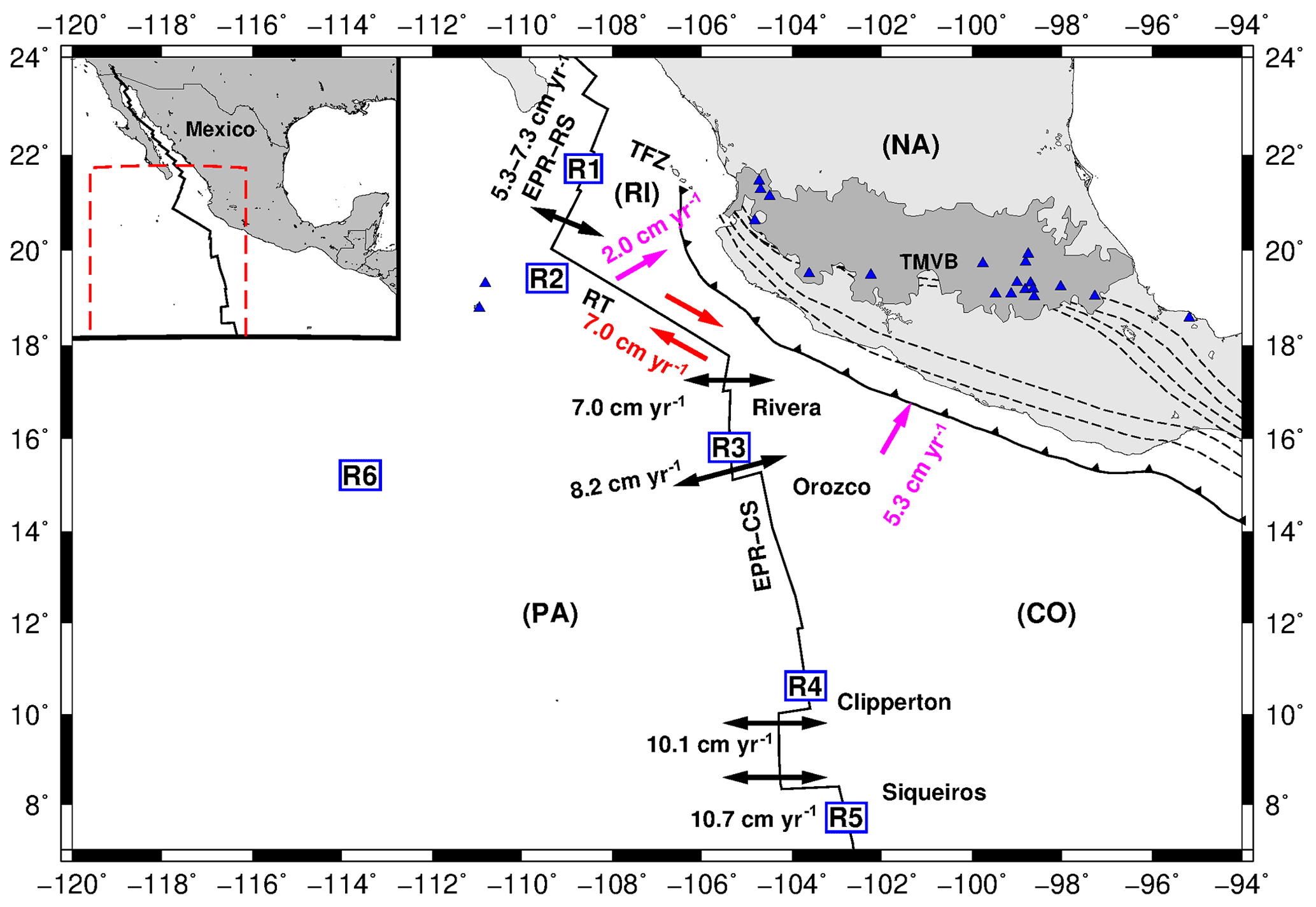
Figure 1Main tectonic features in the oceanic environment off the Pacific coast of Mexico discussed in the text. CO is the Cocos Plate; NA is the North American Plate; PA is the Pacific Plate; RI is the Rivera microplate; TMVB is the Trans-Mexican Volcanic Belt; TFZ is the Tamayo Fracture Zone; EPR-RS is the East Pacific Rise Rivera segment; EPS-CS is the East Pacific Rise Cocos segment; and RT is the Rivera Transform. Blue triangles are volcanoes. Dashed lines show contour lines of the subducted slab. Arrows indicate the motion of the PA, CO, and RI plates. R1 to R6 are the regions in which the study area was divided for analyzing stress and seismicity characteristics. Red number indicates the slipping rates. Pink numbers indicate convergence rates, and black numbers indicate spreading rates.
Table 1Major oceanic earthquakes in Mexico (M>6.8).

(1) Data from the Decade of North American Geology Project (DNAG) of the National Geophysical Data Centre (NGDC) and the Geological Society of America. (2) Pacheco and Sykes (1992). (3) ISC earthquake catalogue. (4) Abe (1981). (5) Global CMT catalogue.
3.1 Data
We used earthquake catalogues of the Mexican National Service (SSN) and the International Seismological Centre (ISC) from 1967 to 2017. Events with no reported magnitude were excluded from our analysis. Reported magnitudes (based on surface, Ms; body, mb; and coda, Mc, waves) were converted to moment magnitude (Mw). The SSN reports Mw for events in Mexico. For the case of the ISC events, Ms and mb were converted to Mw using the scaling relationships of Scordilis (2006). We classified the seismic events into two different categories: (1) intraplate oceanic events (INT, red dots in Fig. 2) and (2) transform fault zone and mid-ocean ridge events (TF-MOR, green dots in Fig. 2). The INT catalogue consists of 177 events with magnitudes in the range of 2.9–6.0. The TF-MOR catalogue includes 2074 earthquakes with magnitudes between 2.7 and 6.9. We also used the Global CMT focal mechanism catalogue (Dziewonski et al., 1981; Ekström et al., 2012) with solutions from 1976 to 2017. For the stress analysis, the focal mechanism catalog was divided into six sub-catalogues shown in Fig. 8 (R1 to R6).
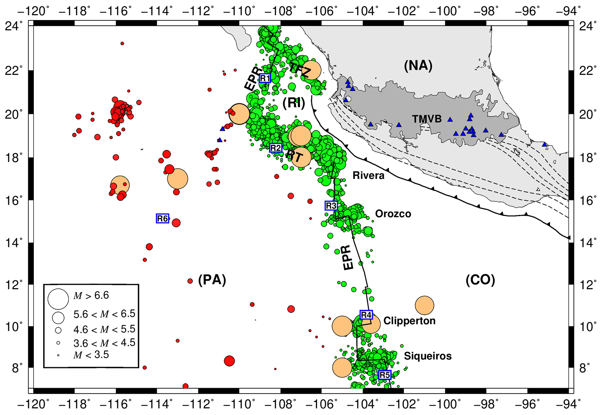
Figure 2Seismicity in the oceanic environment off the Pacific coast of Mexico from 1899 to 2017. The size of the circles represents magnitude. Brown circles are relevant historical earthquakes shown in Table 1 with M>6.8. Red circles are intraplate oceanic events, and green circles are transform fault zone, and mid-ocean ridges earthquakes. Epicenters were compiled from the Mexican National Service (SSN) and the International Seismological Centre (ISC) catalogues.
3.2 Methods
3.2.1 Moment/magnitude earthquake distributions
The Gutenberg–Richter law describes the earthquake magnitude distribution (Ishimoto and Iida, 1939; Gutenberg and Richter, 1944). Mathematically, this law is expressed by the following equation: log, where N(M) is the cumulative number of earthquakes with a magnitude larger than a given magnitude limit (M), the constant b (or b value) describes the slope of the magnitude distribution, and the constant a is proportional to the seismic productivity. The b value describes the distribution of small to large earthquakes in a sample, and it is considered to be specific for a given tectonic environment (e.g., Scholz, 1968; Wyss, 1973; Smith, 1981; Wiemer and Benoit, 1996; Wiemer and Wyss, 2002). In several tectonic environments, b is close to 1 (Utsu, 1961), with deviations affected by many factors. Among them, high thermal gradients and rock heterogeneity (Mogi, 1962; Warren and Latham, 1970) increase the b values. On the contrary, increments in effective and shear stresses (Scholz, 1968; Wyss, 1973; Urbancic et al., 1992) reduce the b value. The b value differs not only between unrelated fault zones (Wesnousky, 1994; Schorlemmer et al., 2005) but also for specific space and time periods (Nuannin et al., 2012). Schorlemmer et al. (2005) found a global dependence of the b value on focal mechanism, which was corroborated at a regional level by Rodríguez-Pérez and Zúñiga (2018). According to those authors, the highest b values correspond to normal-faulting events, followed by strike-slip and thrust earthquakes, respectively. To characterize the b value of oceanic earthquakes and compare the results with other tectonic environments, we calculated the b value with a robust method which has proven its validity in many studies. We estimated the b value by means of the maximum likelihood formulation of Aki (1965) and the completeness magnitude (Mc) employing the maximum curvature method (Wiemer and Wyss, 2000) with the aid of the ZMAP software package (Wiemer, 2001).
As reported by previous authors, seismicity on the mid-ocean transform faults is better represented by a tapered frequency-moment distribution (e.g., Boettcher and McGuire, 2009). This distribution has the following form (Kagan, 1997, 1999; Kagan and Jackson, 2000; Kagan and Schoenberg, 2001; Vere-Jones et al., 2001):
where β is one of the parameters to determine, , where b is the b value, N0 is the cumulative earthquake number over a completeness threshold seismic moment (M0), and Mm is the maximum expected moment. We analyzed if this frequency distribution is suitable for describing the seismicity of oceanic events in Mexico. In order to calculate the tapered Gutenberg–Richter distribution, we used the MATLAB function Get_GR_parameters.m developed by Olive (2016). The tapered Gutenberg–Richter moment distribution is fitted by mens of a least-squares inversion following Frohlich (2007).
3.2.2 Temporal distribution of aftershocks
The frequency distribution of the decrement of earthquake aftershocks is described by the modified Omori's law (Utsu, 1961; Utsu et al., 1995) as
where R(t) is the rate of occurrence of aftershocks within a given magnitude range, t is the time interval from the mainshock, k is the productivity of the aftershock sequence, p is the power-law exponent (p value), and c is the time delay before the onset of the power-law aftershock decay rate. Variations in p values exist for different tectonic regimes and each aftershock sequence. Many authors have related the p value with crustal temperature, heat-flow, or rock heterogeneity in the fault zone. Thus, relevant information can be extracted from these aftershock parameters in order to have a better understating of the rupture process of oceanic earthquakes. As before, we used the ZMAP software package (Wiemer, 2001) for estimating the p value of the aftershock sequence of the 1 May 1997 earthquake (Mw=6.9).
3.2.3 Fragment-asperity model
Alternative statistical models that relate the earthquake magnitude distribution with the rheology of the fault have been proposed. Among them, we have the fragment-asperity model. This model was introduced by Sotolongo-Costa and Posadas (2004) to describe the earthquake dynamics in a Tsallis entropy nonextensive framework (Tsallis, 1988). This model takes into consideration the irregular surfaces of two fault planes in contact and the rock fragments of different shape and sizes that fill the space between them. According to this model, earthquakes are triggered by the interaction along the fault planes of these rock fragments. Considering that large fragments are more difficult to release than small ones, the resulting energy is assumed to be proportional to the volume of the fragment (Telesca, 2010). Silva et al. (2006) improved the model and found a scaling law between the released energy (ε) and the size of asperity fragments (r) by the following proportional factor: ε∝r3. The nonextensive statistics are used to describe the volumetric distribution function of the fragments. A parameter that represents the proportion between ε and r is introduced. This parameter is known as the a value or parameter a (Silva et al., 2006; Telesca, 2010). The parameter a is defined using a volumetric distribution function of the fragments applying the maximum entropy principle for the Tsallis entropy (for details in the mathematical expressions see Silva et al., 2006; Telesca, 2010). The magnitude cumulative distribution function becomes
where N is the total number of earthquakes; N (>M) represents the number of events with magnitude larger than M; a is a proportionality parameter between ε and r, and q is the nonextensivity parameter. K is defined as K=2M (Silva et al., 2006) or K=M (Telesca, 2011). The magnitude (M) is related to ε by the following relation: log(ε) (Silva et al., 2006). Telesca (2011) considered that the relation between ε and M is given by log(ε). Neither of the two models is preferred over the other. We used both models in order to quantify the variability in the nonextensive parameters. According to Telesca (2010), the physical meaning of the q parameter consists in that it provides information about the scale of interactions. It means that if q is close to 1, the physical state is close to the equilibrium. As a result, few earthquakes are expected. On the other hand, as q rises, the physical state goes away from the equilibrium state, this implies that the fault planes are able to generate more earthquakes, thus resulting in an increment in the seismic activity (Telesca, 2009, 2011). The physical meaning of the a value lies in the fact that it provides a measure of the energy density. It means that the a value is large if the energy released is large (Telesca, 2011). For example, high a values are expected when the events with the highest magnitude take place. Previous studies have shown that the q value ranges mainly from 1.50 to 1.70 (Vilar et al., 2007; Vallianatos, 2009; Rodríguez-Pérez and Zúñiga, 2017, among others). We obtained the a and q parameters by minimizing the root mean square error (RMS) with the Nelder–Mead method (Nelder and Mead, 1965).
3.2.4 Stress inversion
Focal mechanisms are reliable indicators of the state of stress in a tectonic region. In order to study the regional stress field for oceanic earthquakes, we performed stress tensor inversion from focal mechanisms reported in the Global CMT catalogue (Dziewonski et al., 1981; Ekström et al., 2012) with the iterative joint inversion developed by Vavryčuk (2014). From the stress inversion, we obtained the orientation of the principal stress axes σ1, σ2, and σ3 (where ) and the stress ratio R. We now briefly explain each method. The first method (the iterative joint inversion) provides an accurate estimation of R and stress orientations (Vavryčuk, 2014). In this method, the ratio is defined as (Gephart and Forsyth, 1984). A fault instability constraint is applied, and the fault is identified with that nodal plane, which is more unstable and thus more susceptible to faulting (Vavryčuk, 2014). By incorporating a fault instability constraint into the inversion, an iterative procedure is imposed. The uncertainties are determined as the differences between the inverted results considering noisy data (Vavryčuk, 2014). The stress inversion was carried out with the STRESSINVERSE software developed by Vavryčuk (2014). The maximum horizontal stress (SHmax) was calculated using the formulation of Lund and Townend (2007). The stress inversion was performed for each of the six different regions shown in Fig. 7.
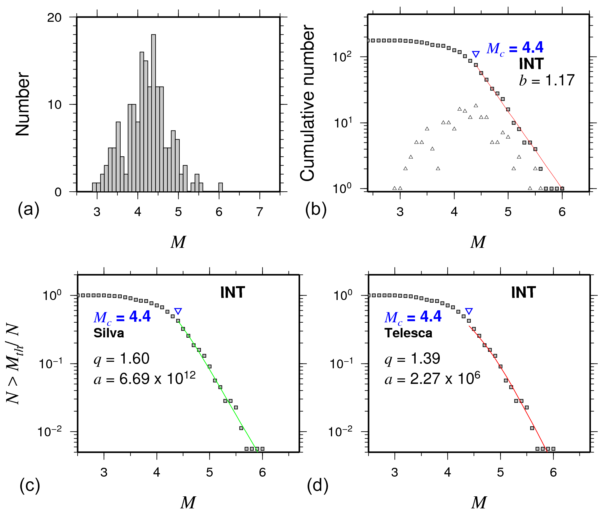
Figure 3Main statistical characteristics for intraplate oceanic events (INT). (a) Magnitude earthquake histogram; (b) frequency–magnitude distributions with Mc and b values. (c, d) The normalized cumulative number of events as function of magnitude for intraplate oceanic events (INT). Color curves show the best fit for the nonextensivity parameters q and a for the Telesca (2010) (red lines) and the Silva (2006) (green lines) models, respectively.
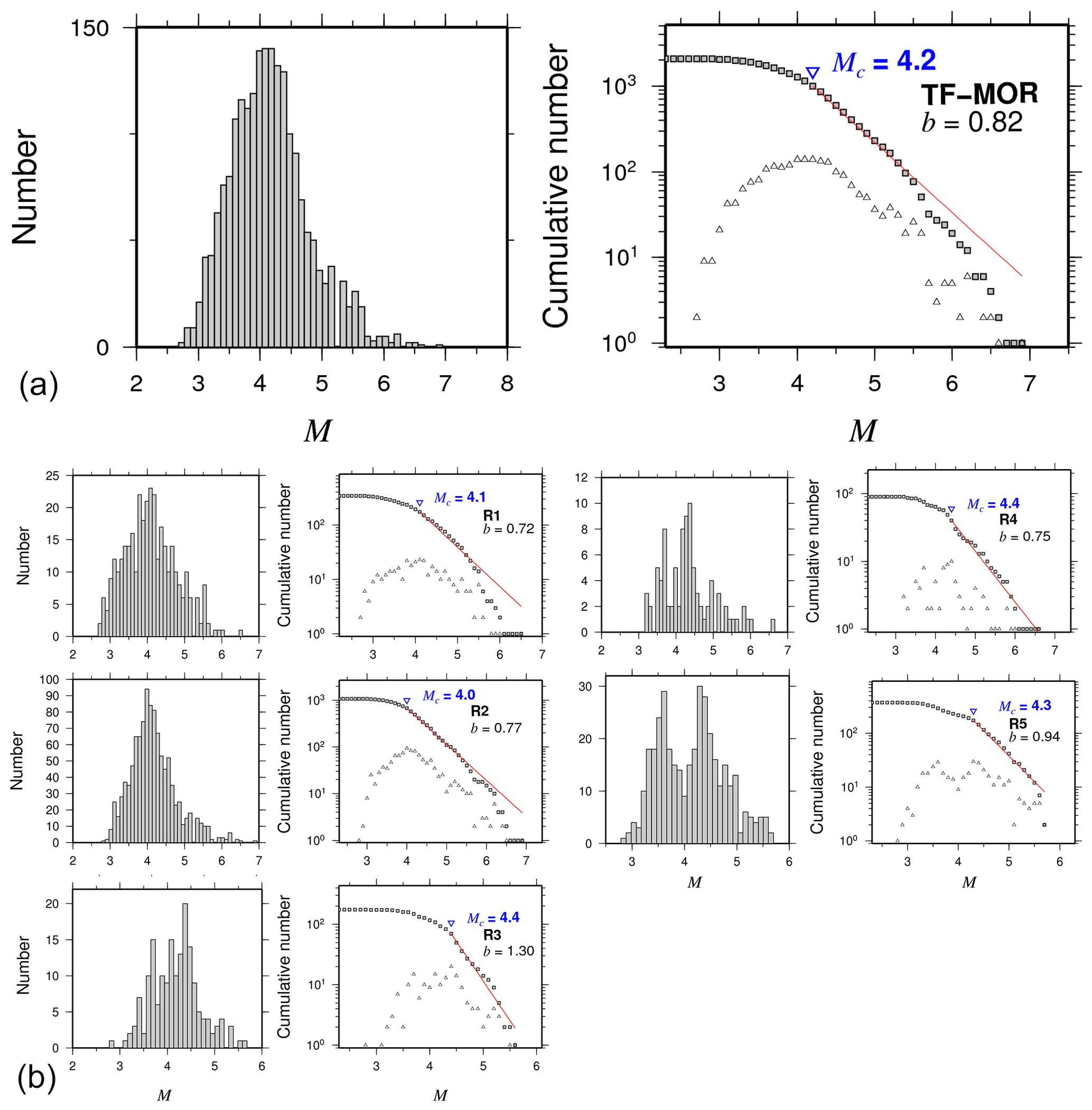
Figure 4(a) Main statistical characteristics for the transform fault zone and mid-ocean ridge (TF-MOR) events (regions R1 to R5). (b) Magnitude earthquake histograms and frequency–magnitude distributions with Mc and b values for each of the different subregions shown in Fig. 8.
There is a large span of b values (Table 2) which nevertheless sheds light on the seismicity characteristics of oceanic earthquakes in Mexico. INT events exhibit higher b values and Mc than TF-MOR events (Figs. 3, 4a and Table 2). In particular, TF-MOR events also show local b-value variations in the range of 0.72–1.30 (Fig. 4b) for each of the subregions R1 to R5 (Table 2). Previous studies had shown large fluctuations in b values of oceanic events. For example, Tolstoy et al. (2001) reported b values of about 1.5 associated with volcanic activity in the Gakkel Ridge. Läderach (2011) reported b values of 1.28 in the Southwest Indian Ridge. In a global study, Molchan et al. (1997) estimated the b value for mid-ocean and transform zones, obtaining values of the following interval 0.97–1.47. In general, our b-value estimates agree with reported b values in previous studies. On the other hand, our results showed that Mc for oceanic events is higher than reported Mc for the subduction zone and continental regions of Mexico, which reflects the capability of the global and regional networks to appropriately register events in that region. The magnitude completeness for oceanic earthquakes differs for different parts of the world, but in most cases, it is in the range of 4.0–5.0 on average considering most of the global catalogues.
Table 2Statistical parameters.
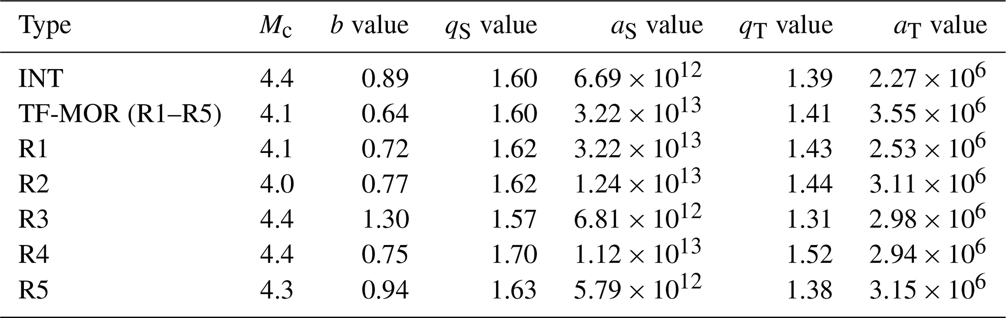
INT are intraplate oceanic events; TF-MOR are transform fault zone and mid-ocean ridge events; Mc is the completeness magnitude; b is the slope of the Gutenberg–Richter distribution; qS and aS and qT and aT are the nonextensive parameters based on Silva et al. (2006) and Telesca (2011), respectively.
Our results also showed that transform fault zone and mid-ocean ridge events follow a tapered Gutenberg–Richter distribution, as suggested in previous studies (Boettcher and McGuire, 2009). The tapered Gutenberg–Richter distribution was fitted with the following parameters: β=0.64 and an estimated corner magnitude of Mm=6.7 (Fig. 5a). These results are in agreement with previous studies such as that of Bird et al. (2002), which studied the tapered Gutenberg–Richter distribution for spreading ridges and oceanic transform faults based on global data, obtaining a β value of about 0.67 for both types of events. They reported that Mm varies from 5.8 to 6.6–7.1 for mid-ocean ridge and transform faults, respectively. The results for the nonextensive parameters are shown in Table 2. We found higher q values for TF-MOR events than for INT events (Fig. 5), meaning that TF-MOR events are farther from the equilibrium than INT events. The results showed a better fit for cumulative distribution functions using the Telesca model for TF-MOR and each of the regions (Fig. 6). In regions R1-R5, our results showed that q varies from 1.31 to 1.52 and from 1.57 to 1.63 using Telesca's and Silva's models, respectively. In the case of subduction zones, the q value can vary from 1.35 to 1.70. For example, in the Hellenic Subduction Zone, q is in the range of 1.35–1.55 (Papadakis et al., 2013); in the Mexican Subduction Zone, Valverde-Esparza et al. (2012) found that q varies from 1.63 to 1.70. Thus, our results conform to values obtained in regional studies.
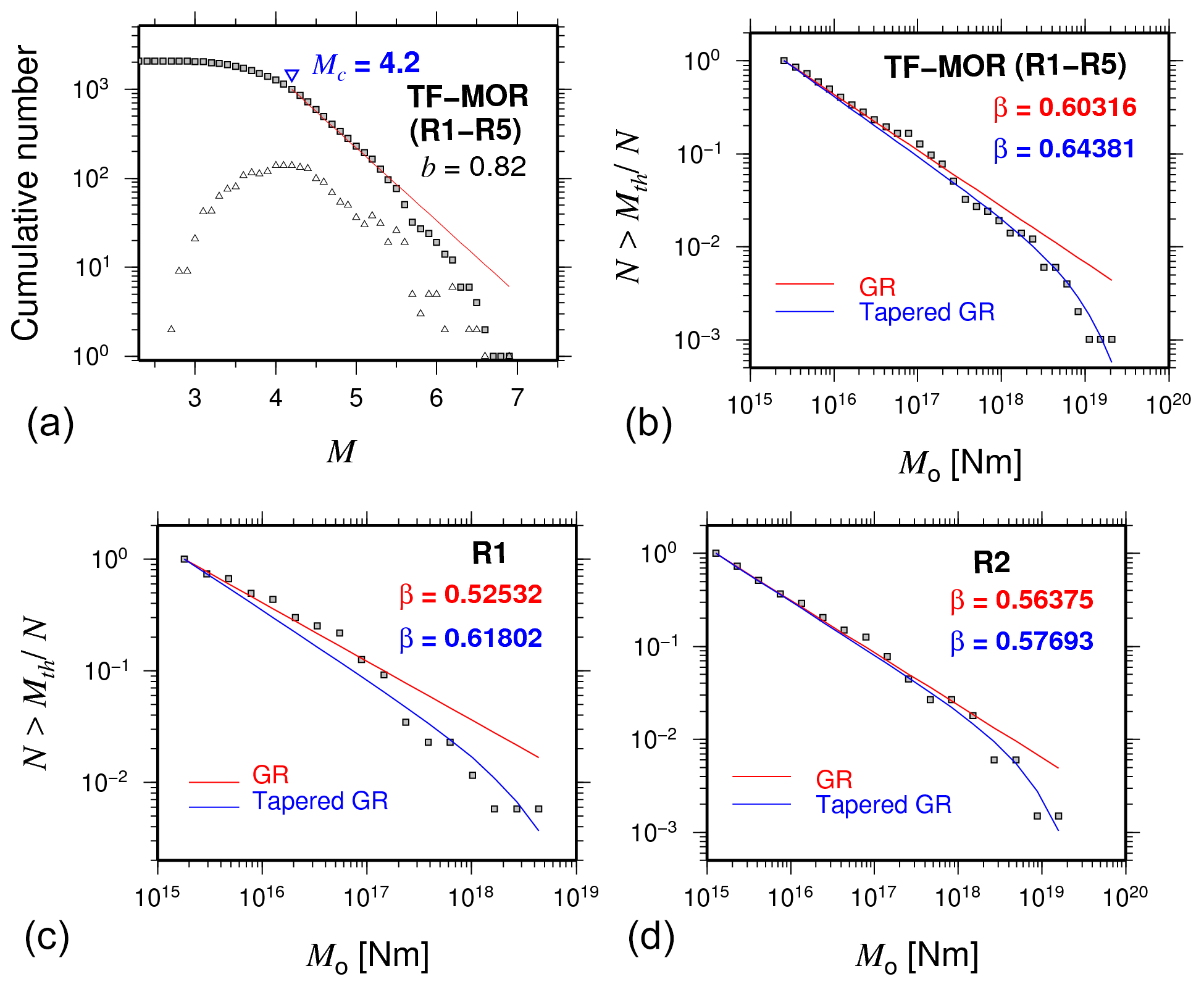
Figure 5(a, b) The cumulative annual seismic moment frequency distribution for the transform fault zone and mid-ocean ridge (TF-MOR) events (regions R1 to R5). The blue lines are the moment, tapered Gutenberg–Richter distributions. The red lines represent the ordinary moment Gutenberg–Richter distributions. (c, d) The subregions that do not follow an ordinary moment Gutenberg–Richter distribution are subregions R1 and R2.
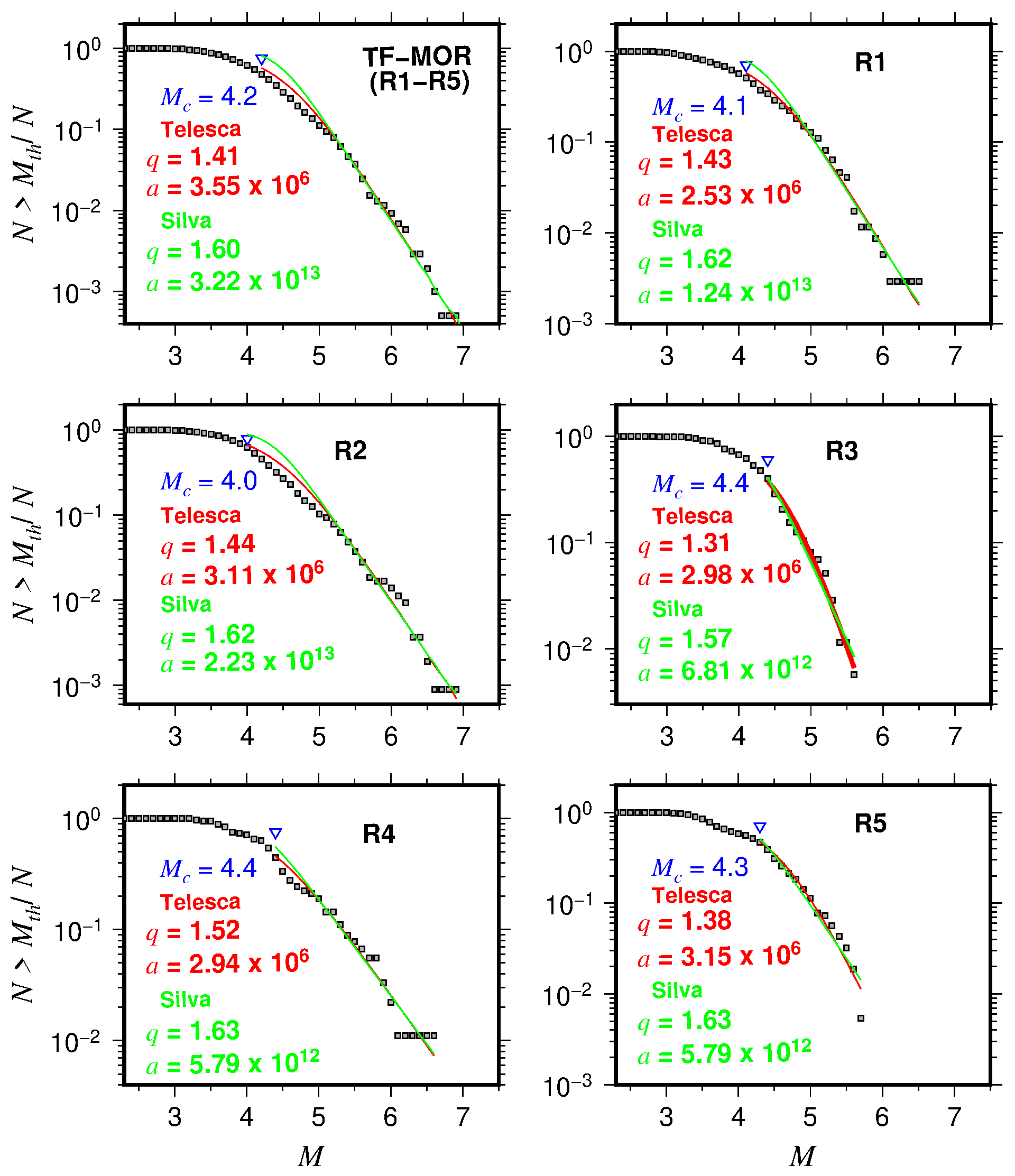
Figure 6The normalized cumulative number of events as function of magnitude for the transform fault zone and mid-ocean ridge (TF-MOR) events. Blue triangles show the completeness magnitude (Mc). Red curves show the best fit for the nonextensivity parameters q and a for Telesca's (2010) model (red lines). Green curves show the best fit for the nonextensivity parameters q and a for Silva's (2010) model (green lines).
The analysis of the aftershock sequence of the 1 May 1997 earthquake (Mw=6.9), yielded a p value of 0.67±0.33 (Table 3). The magnitude of the largest aftershock of the 1997 event was Mw=5.3 (Table 3). Oceanic strike-slip events seem to have lower p values than mid-ocean ridge events. For example, Bohnenstiehl et al. (2004) found a p value of 0.95 for the 15 July 2003 (Mw=7.6) central Indian Ridge strike-slip event. For the Siqueiros, Discovery, and western Blanco transforms, the p value varies from 0.94 to 1.29 (Bohnenstiehl et al., 2002). Davis and Frohlich (1991) determined a p value of 0.928±0.024 for the combined ridge and transform environments. Our results fall within the range of global studies that showed that the p value varies from 0.6 to 2.5 (Utsu et al., 1995). We also reported a c close to 0 for the aftershock sequence of the 1 May 1997 (Mw=6.9) (Table 3). Shcherbakov et al. (2004) found that the parameter c of the Omori's law decreases as the magnitude of events considered increases. According to the study, this observation is due to the effect of an undercount of small aftershocks in short time periods. This provides an explanation for our result of c∼0 because of the limited magnitude detection reported in the regional and global catalogues used.
Table 3Aftershocks characteristics of 1 May 1997 event.
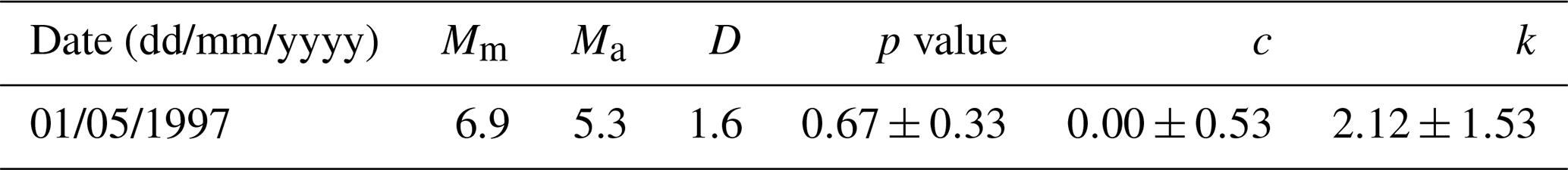
Mm is the magnitude of the mainshock; Ma is the magnitude of the largest aftershock; D is the difference in magnitudes of the mainshock and its largest aftershock; p, c, and k are the coefficients of Omori's law.
We classified the focal mechanisms used in the stress inversion into seven categories: (1) reverse, R; (2) reverse with lateral component, R-SS; (3) strike-slip with reverse component, SS-R; (4) strike-slip, SS; (5) strike-slip with normal component, SS-N; (6) normal with lateral component, N-SS; and (7) normal, N (Fig. 7). This classification was performed to identify the dominant type of faulting for each subregion. Region R1 is composed of strike-slip (70.3 %), strike-slip with normal and reverse components (21.6 % and 5.4 %, respectively), and normal-faulting (2.7 %) focal mechanisms (Fig. 7b). Region R2 exhibits the following focal mechanism distribution: strike-slip (82.4 %) and strike-slip with normal and reverse components (9.5 % and 8.1 %, respectively) (Fig. 7b). In region R3, the focal mechanism classification shows the following distribution: strike-slip (62.5 %), strike-slip with normal component (25 %), normal-faulting with strike-slip component (6.3 %), and reverse (6.3 %) (Fig. 7b). Region R3 consists of strike-slip (70.8 %), strike-slip with normal and reverse components (8.3 % and 16.7 %, respectively), and reverse earthquakes (4.2 %) (Fig. 7b). Region R5 exhibits the following focal mechanism distribution: strike-slip (53 %), strike-slip with normal and reverse components (23.5 % and 17.6 %, respectively), and reverse (5.9 %). For the case of earthquakes in R6, the classification shows the following distribution: normal (83.3 %) and normal-faulting with strike-slip component (16.7 %) (Fig. 7b).
Table 4Stress inversion results.
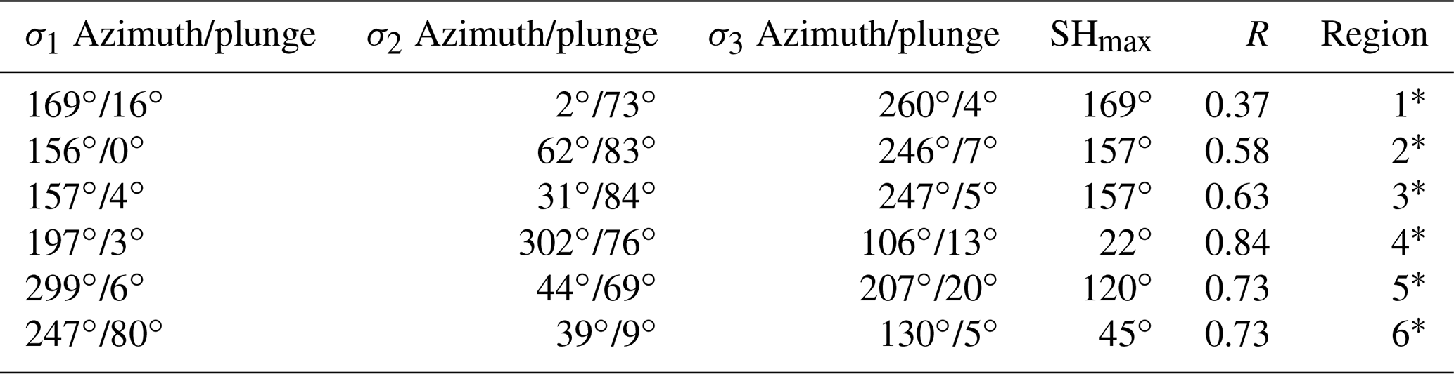
Stress ratio is defined by ; * stress inversion based on Vavryčuk (2014) and Lund and Townend (2007). Location of the regions are shown in Fig. 1.
Table 4 summarizes the results from the stress inversion. Based on the orientation of stress axes, a dynamical description of the tectonics of the oceanic earthquakes in Mexico can be carried out. A quantitative comparison with other oceanic regions is discussed in what follows. Region R6 is only dominated by N and N-SS earthquakes (Fig. 8). In regions R4 and R5, stress results showed moderate similarities. The differences in these regions may also be related to the variability in focal mechanisms (here we have SS, SS-N, SS-R, and to a lesser extent R events) (Fig. 8). Variations are very significant in regions R1 to R3 (particularly in σ2) (Table 4). These regions also showed different types of events: SS, SS-N, and SS-R for R1; SS, SS-N, and SS-R for R2; and SS, SS-N, N-SS, and R for R3 (Fig. 8). In these regions, strike-slip earthquakes are the dominant type of faulting. Events with unusual mechanisms have also been reported in other oceanic regions. According to Wolfe et al. (1993), most of the anomalous seismic activity is associated with mislocations, complex fault geometry, or large structural features with an influence on the slip of the fault. DeMets and Stein (1990) showed that the strike direction and earthquake slip vectors in the Rivera Transform are rotated clockwise from the expected direction of the Pacific–Rivera Euler vector. This deviation can be the result of morphologic features resulting in unusual patterns of epicenters and focal mechanisms.
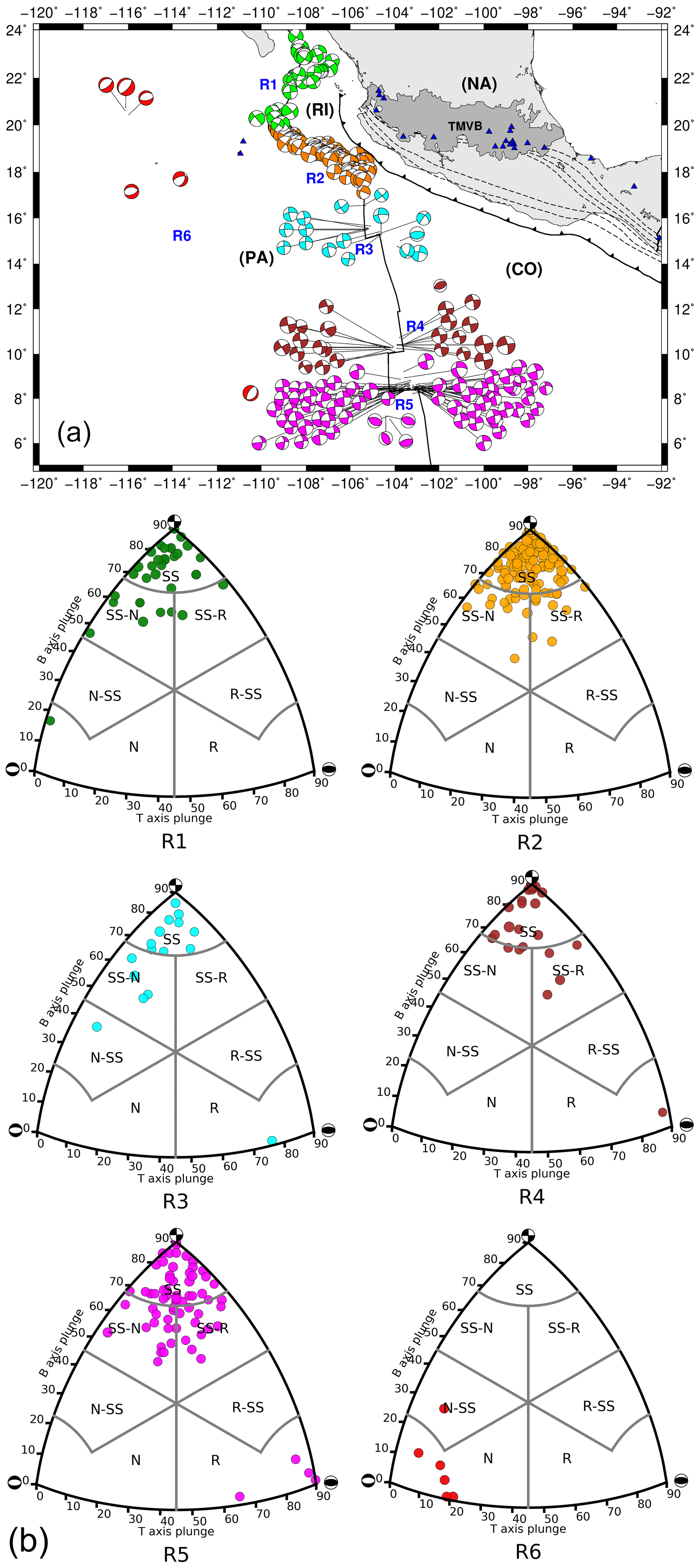
Figure 7Focal mechanism solutions of oceanic earthquakes in Mexico reported by the Global CMT catalogue from 1976 to 2017. (a) Focal mechanisms are divided into six regions (R1 to R6) for the stress inversion analysis. (b) Focal mechanism classification based on the Kaverina et al. (1996) projection technique implemented by Álvarez-Gómez (2015): reverse, reverse with lateral component, strike-slip with reverse component, strike-slip, strike-slip with normal component, normal with lateral component, and normal (R, R-SS, SS-R, SS, SS-N, N-SS, and N, respectively).
In the case of the East Pacific Rise Rivera segment (region R1), σ2 is almost vertical, and SHmax is ∼170∘, suggesting a strike-slip regime (Table 4). The main orientations of the P axes are in the N–S, NW–SE, and E–W directions. The orientations of the P axes are NW–SE and, to a lesser extent, E–W directions (Fig. 9). For the case of the Rivera Transform (region R2), σ2 is quasi vertical, and the SHmax is 157∘, suggesting a strike-slip regime. The orientation of the P axes is in the NW–SE direction, and the orientation is in the NE–SW direction for the T axis. In region R3, σ2 is almost vertical, and the SHmax is also 157∘, suggesting a strike-slip regime. The orientation of the P axis is in the NW–SE direction. The main orientation of the T axes is NE–SW, but E–W directions occur as well. For the region R4, σ2 is 76, and the SHmax is 22∘, suggesting a strike-slip regime. The predominant orientations of the P and T axes are NE–SW and NW–SE, respectively. In R5, σ2 is from 69∘, and the SHmax is 120∘, suggesting a strike-slip regime. The main orientation of the P axes is NW–SE, while that of the T axis is NE–SW. In R6, the principal axes are related to a normal fault regime. σ1 is almost vertical, and the SHmax is ∼45∘. The orientation of the T axes is in the NW–SE direction. The Mohr circle diagram showed that most of the studied events are clustered along the outer Mohr's circle in the area of validity of the Mohr–Coulomb failure criterion (Fig. 9). Reported focal mechanisms confirm Sykes's model for mid-ocean ridges (Sykes, 1967), where events in transform zones tend to have strike-slip mechanisms, while ridge crest events have mainly normal faults. The obtained orientation of the principal axes supports this model.
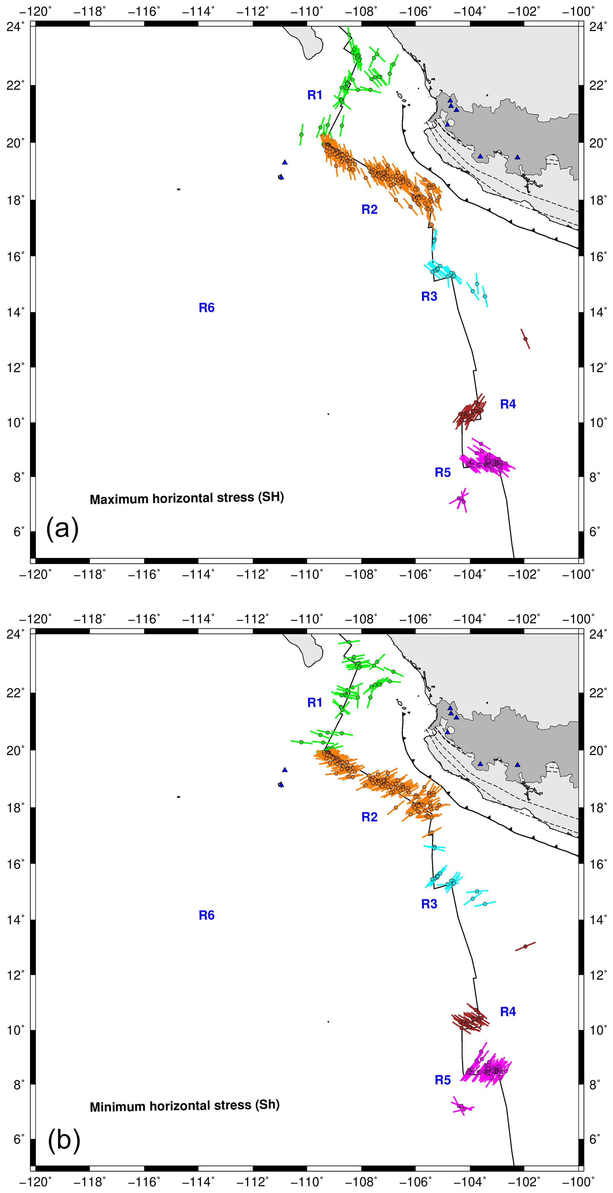
Figure 8Orientation of horizontal axes. (a) Maximum horizontal stresses (SH); (b) Minimum horizontal stresses (Sh).
One of the main problems for studying oceanic seismicity is that the epicenters are located far from most of the recording stations in mainland Mexico. This has a direct effect on the earthquake magnitude distributions (Mc and b value). We first discuss the magnitude completeness of oceanic earthquakes. Global studies showed that the magnitude completeness for oceanic earthquakes is in the range of 4.0–5.0. Our results are in agreement with these global studies. However, as expected, several microseismic surveys which have been conducted in different oceanic environments (e.g., Smith et al., 2003; Simão et al., 2010; McGuire et al., 2012, among others) can yield lower-magnitude thresholds. As a result of these studies, precise hypocenter locations and earthquake distributions with a broader magnitude range were obtained. Thus, lower Mc has been reported for studies based on microseismic surveys. For example, in the Mid-Atlantic Ridge, Mc∼3.0 with several smaller events (Mw<2.5) were reported (Bohnenstiehl et al., 2002; Smith et al., 2002, 2003).
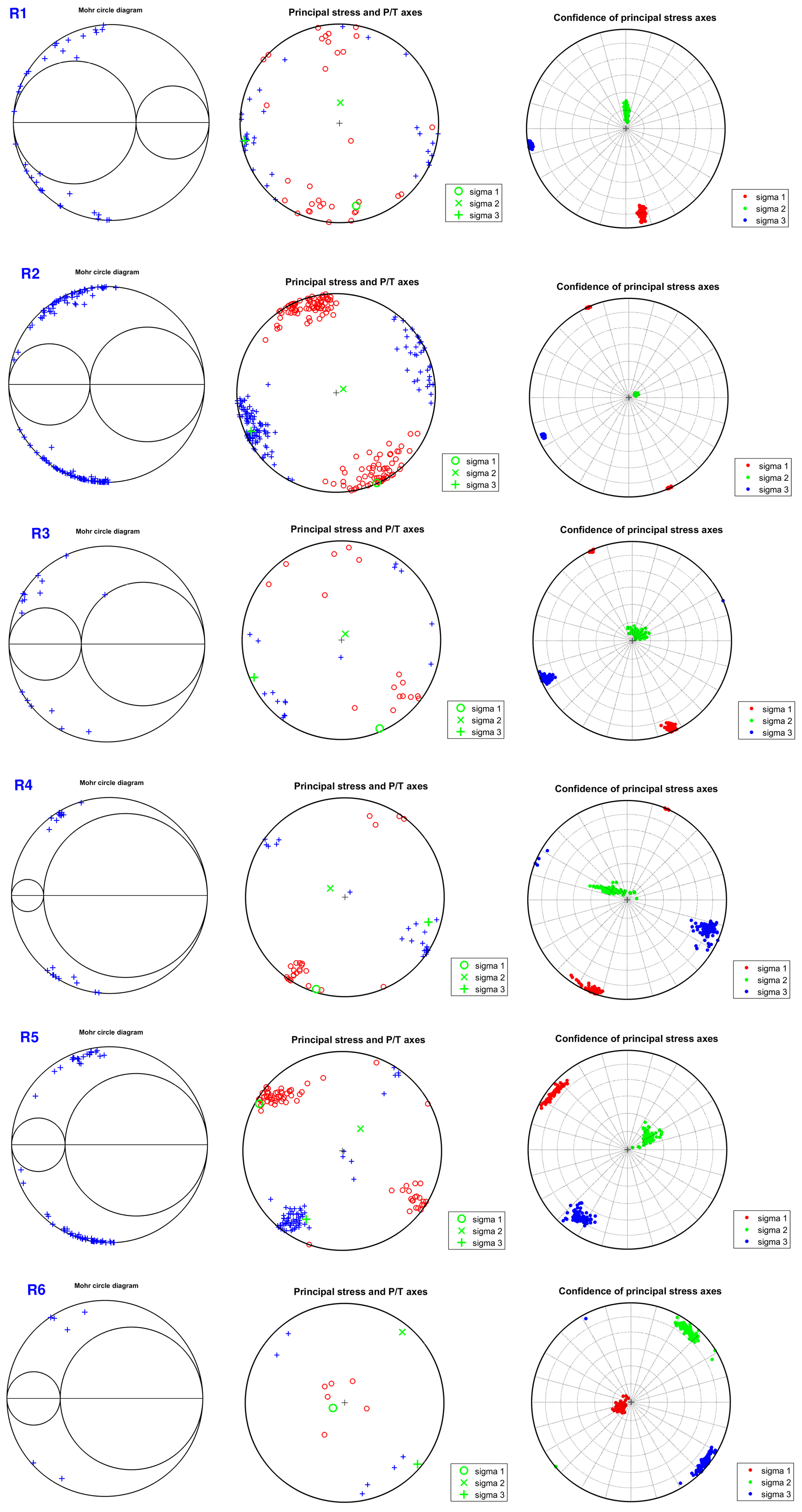
Figure 9Mohr circle diagrams for all the regions (left column). P and T axes distributions for all the regions (right column). Red circles represent pressure, while blue crosses represent tension.
Another factor that has to be discussed is the accuracy in the location of the epicenters. The location uncertainty plays an important role when earthquakes are assigned to an intraplate or a mid-ocean ridge/transform fault environment. For example, some studies reported that for faults located at 4S on the EPR, teleseismic locations could be off by as much as 50 km (McGuire, 2008; Wolfson-Schwehr, 2014). As a consequence, some TF-MOR events are probably classified as INT events and vice-versa (for example, epicenters in color in Fig. 2). Some events located in the Tamayo Fracture Zone close to the Rivera Subduction Zone may also be misidentified. This mislocation effect introduces uncertainties in the estimation of the statistical parameters useful for understanding the tectonics of the region. In order to have precise locations and avoid mislocation, ocean-bottom seismometers off the Mexican coast would be needed. Being aware of this, one should avoid over-interpretation of the results. Local monitoring of oceanic events represents an improvement of more than an order of magnitude relative to the regional and teleseismic detection levels.
Previous studies also showed that the seismicity near oceanic transform faults that connect mid-ocean ridges may be thermally controlled (Abercrombie and Ekström, 2001; Boettcher et al., 2007). The thermal effect is most evident in the seismogenic zone. It is essential to mention that faults along the middle and southern segments of the EPR are shorter and faster slipping. The faster slip rates and shorter fault lengths result in narrower seismogenic zones because the thermal structure is shallow. On the other hand, the Rivera Transform is longer and has a slower slip rate, resulting in a wider seismogenic zone. However, heat is not the only factor that regulates seismicity, because the largest events break a small part of the rupture areas predicted by thermal models (Boettcher and Jordan, 2004; Roland et al., 2010). Thus, most slip occurs without producing large earthquakes (Goslin, 1999; Boettcher and Jordan, 2004; Roland et al., 2010). This can explain the occurrence of a few events with M>6.5 in the Rivera Transform. According to McGuire et al. (2012), the apparent lack of large events on mid-ocean ridge transform faults may also be related to the heterogeneity of materials on the fault plane. The maximum magnitude for transform fault events on the East Pacific Rise (in the latitude interval of 3∘ < Lat < 5∘) is about 6.5 (McGuire et al., 2005). On the other hand, earthquakes in the Rivera Transform and on the northern segment of the East Pacific Rise (in Mexico) have relative larger magnitudes (M>6.8) based on reported seismicity in different catalogues (Fig. 1). This highlights a differentiation between the middle and southern and northern segments of the East Pacific Rise.
A further aspect of the analysis of oceanic earthquakes is their capacity to generate aftershocks as well as the their occurrence, duration, and magnitude. Earthquake statistical studies showed that large oceanic events in transform faults, fracture zones, and intraplate regions release low energy levels in their aftershock sequences (Houston et al., 1993; Boettcher and Jordan, 2001; Antolik et al., 2006). Boettcher et al. (2012) found that earthquakes on transform faults have an order of magnitude fewer aftershocks than intraplate events. According to some authors, a low aftershock-to-mainshock energy ratio indicates an efficient rupture or complete stress drop in the mainshock presupposing a weak fault (Hwang and Kanamori, 1992; Velasco et al., 2000). Many factors can affect the aftershock productivity. For example, the age of the lithosphere and the heat flux have a direct influence on the rock strength (Antolik et al., 2006), thus, explaining the low energy release in the aftershock sequence of oceanic events. The observed low aftershock energy seems to be a common feature of oceanic earthquakes (Antolik et al., 2006). In this regard, we studied the 1 May 1997 (Mw=6.9) strike-slip event in the Rivera Transform and its largest aftershock (Mw=5.3). By considering the energy magnitude as log , we obtain that the energy of the mainshock is 1.41×10¹⁵ Nm, and the energy of the largest aftershock is 5.62×10¹⁵ Nm, resulting in an aftershock-to-mainshock energy ratio of 0.003. This value is considered as low and representative of strike-slip events, as shown by the comparison with the results reported by Velasco et al. (2000).
A similar analysis comes from Båth's law by considering the magnitude difference between the mainshock and the largest aftershock. We determined that the magnitude difference for the 1997 event is 1.6, which is higher than the theoretical value of 1.2. Both magnitude difference and the aftershock-to-mainshock energy ratio showed large scatter (e.g., Velasco et al., 2000; Utsu, 2002), and results ought to be taken with caution. The aftershock decay rate is the product of the strain relaxation around the rupture plane. Aftershock studies have shown that oceanic ridges are prone to having larger p values than those of subduction zone regimes due to the high temperature of the oceanic crust, which results in rapid strain release (Kisslinger, 1996; Rabinowitz and Steinberg, 1998; Klein et al., 2006). According to previous studies, extremely high p values (p>2) and short aftershock durations are related to high temperatures (Bohnenstiehl et al., 2002; Simão et al., 2010) and/or migration of hydrothermal fluids (Goslin et al., 2005). We found a p value of 0.67±0.33 for the 1 May 1997 (Mw=6.9) strike-slip event in the Rivera Transform. This p value is consistent with other oceanic regions, but it does not seem to conform to a high-temperature regime.
Regarding the magnitude distribution of oceanic events, our b-value estimates are in agreement with global oceanic studies but differ from local studies. For example, along the East Pacific Rise (in the latitude interval of 5∘ N < Lat < 9.90∘ N), b-value estimations fluctuate from 1.10 to 2.50 (Bohnenstiehl et al., 2008). Bohnenstiehl et al. (2008) determined the b value of 9000 microearthquakes with magnitudes in the range of −1.5–1.0 located in the southern part of our study zone. Due to this overlap, we compare their results with our results for region R5. For this region, we obtained a b value of 0.94 with a Mc of 4.2, while they found that the b value approaches 2.5 at very shallow depths (< 0.3 km) (with ). At depths of 0.5–1.5 km, the b values drop to a value of 1.10 (with ). According to Bohnenstiehl et al. (2008) at very shallow depths, the uppermost oceanic crust is structurally heterogeneous because of the extrusion of lava and the repeated emplacement of sheeted dikes. As a consequence, there is a large proportion of small versus large earthquakes resulting in high b values. The b values decrease with depth due to the decreasing heterogeneity and/or changes in ambient stress levels. Considering that events in our catalogue for R5 occur at a different depth interval, and assuming the decreasing heterogeneity, fewer magnitude events would be expected (reducing the b value). Another explanation for the differences between our results and the results of Bohnenstiehl et al. (2008) is that the magnitude ranges of the earthquake catalogues are extremely different. This highlights how the b value is affected by magnitude completeness.
Statistical studies suggested that the β value mainly takes values between 0.60 and 0.70 for a global range (Kagan, 2002). Our estimates of β agree with global oceanic studies. It is essential to discuss the tectonic implications of this parameter. Bird et al. (2002) also found a dependence of β value on the relative plate velocity. According to them, the β value is higher (with Mm=7.1) when the velocity is < 36 mm yr−1 than when the velocity is > 67 mm yr−1 (with Mm=6.6) for spreading ridges and oceanic transform faults, respectively. These observations are in agreement with our estimate of β=0.64 and Mm of 6.6 for oceanic earthquakes in Mexico (Fig. 5). For intraplate events, we obtained a β>0.70. According to Kagan (2010), β values > 0.70 may be related to the mix of earthquake populations with different maximum magnitudes (Mm). In the case of intraplate events, we associated the somewhat high β values with the mix of some intraplate and mid-ocean–transform events. This could be related to incorrect hypocenter locations due to the difficulty of precisely locating oceanic events by the land-based networks.
The seismicity models based on nonextensivity consider the interaction of two irregular fault surfaces (asperities) and rock fragments filling them. However, these models differ in their assumption of how energy is stored in the fragments and the asperities. This difference is expressed through the constant a, which represents the proportionality between the released energy E and the fragment size r. This explains the difference in a parameter between Telesca's and Silva's models (Fig. 5). Both models showed that a for TF-MOR is higher than a for the INT events (Fig. 5). This implies that more energy is released for TF-MOR earthquakes. On the other hand, the q value indicates if the physical state of a seismic area moves away from equilibrium. The physical state is at equilibrium when q is equal to 1, and as q increases, the system is in an instability state in which a more significant amount of seismic energy is released.
Finally, we discuss the focal mechanisms and the calculated state of stress for oceanic earthquakes in Mexico. Focal mechanisms provide useful information about the structure and settings of faults and can describe the crustal stress field in which earthquakes take place. Our analysis is limited because we only used focal mechanisms based on teleseismic data. The teleseismic detection threshold for oceanic events in the East Pacific Rise is dependent on the region of the EPR. For example, Riedesel et al. (1982) report a magnitude detection threshold in the range of 4.0–5.0. For the Quebrada, Discovery, and Gofar faults, the CMT catalogue is only complete to MW=5.4. (McGuire, 2008; Wolfson-Schwehr et al., 2014). Another limitation of our study is that we combine different types of earthquakes into a single region, resulting in inaccurate estimations of the stress state for that specific region. Under these circumstances, our study provides information on the stress field of major structures or the stress associated with the dominant types of earthquakes.
In oceanic environments, the largest magnitude events along transform fault or intraplate earthquakes usually show strike-slip mechanisms (Wiens and Stein, 1984; Kawasaki et al., 1985). In the areas adjacent to the oceanic ridges where the oceanic lithosphere is young, Wiens and Stein (1984) reported a large variety of focal mechanisms and stress orientations. For example, in the East Pacific Rise, in the Mexican territory, Wiens and Stein (1984) reported thrust and normal mechanism solutions for near ridge intraplate seismicity. This explains the strike-slip with normal components, as well as thrust events in regions R3, R4, and R5 (Fig. 7). In R3 and R4 (Fig. 7), the maximum horizontal axes (compression) of thrust events show a preferred orientation perpendicular to the spreading direction. On the other hand, in region R5 (Fig. 7), the compression axes, showed a weak preferred alignment with respect to the spreading direction. In the Rivera Transform, focal mechanisms showed right lateral strike-slip motion implying oblique horizontal stresses (Fig. 7). Although most of the events in the Rivera Transform (R2 in Fig. 7) are strike-slip events, some events with unusual mechanisms have been reported (normal faulting events) (Wolfe et al., 1993). Normal faulting events may be related to extensional offsets or internal deformation of the Rivera Plate (Wolfe et al., 1993).
We analyzed the seismicity of oceanic events in the Pacific oceanic regime of Mexico. Oceanic earthquakes were classified into two different categories: intraplate oceanic (INT) and transform fault zone and mid-ocean ridge (TF-MOR) events, respectively. We conducted a stress state estimation for the different regions. Because of the combination of different types of earthquakes into the regions, our results only provide information on the stress field of major structures or the stress associated with the dominant types of earthquakes. It is important to be aware of this limitation in order to avoid an over-interpretation of the results. TF-MOR events have strike-slip, strike-slip with normal and reverse components, normal and normal-faulting with the strike-slip component, and reverse focal mechanisms. On the other hand, INT events have only normal and normal-faulting with strike-slip component focal mechanisms. The stress field from INT and TF-MOR events agree with global studies. Regarding the aftershock productivity, we found that the aftershock decay rate of the 1 May 1997 (Mw=6.9) strike-slip event in the Rivera Transform is also consistent with oceanic p-value estimations. Despite the limitation of the catalogues used, our results provided a comprehensive insight into the seismicity of oceanic environments. The main problem is the location uncertainty and mislabeling of the earthquakes. The b value for INT events (1.17) is higher than that for TF-MOR events (0.82). Our b-value estimations are in agreement with other regional studies but differ from b-value estimates based on microseismicity studies. Our b-value estimates for mid-ocean ridge/transform fault environments are lower (0.72<b<1.30) than those derived from microseismicity studies (1.1<b<2.5). Our results also showed that TF-MOR events mostly follow a tapered Gutenberg–Richter distribution.
From the nonextensivity analysis, we observed that TF-MOR events are farther from the equilibrium than INT events. Thus high q values take place in mid-ocean ridges and transform fault zones. This means that mid-ocean ridge and transform faults are able to produce more seismicity. Low q values are also reported during relatively quiet periods, characterized mainly by the occurrence of small-magnitude events. This can be an explanation for the low q values of regions R1 and R5. Our results also showed that a values are higher for TF-MOR events than for INT events using both models. This implies that more earthquakes with larger magnitude occur (or more energy is released) in mid-ocean ridge/transform fault environments than in an oceanic continental environment. Telesca's model fits better with the cumulative magnitude distribution functions making a better option to study the oceanic seismicity in Mexico.
Generic Mapping Tools (GMT5) is available at http://gmt.soest.hawaii.edu/, last access: 13 January 2020. Get_GR_parameters.m is available at https://jaolive.weebly.com/codes.html, last access: 23 December 2019. FMC is available at https://josealvarezgomez.wordpress.com, last access: 13 January 2020. Stressinverse_1.1 is available at https://www.ig.cas.cz/en/stress-inverse/, last access: 13 January 2020. ZMAP is available at http://www.seismo.ethz.ch/en/research-and-teaching/products-software/software/ZMAP/, last access: 13 January 2020.
Earthquake catalogues data is available at Earthquake catalogue of the Servico Sismológico Nacional, http://www.ssn.unam.mx/, last access: 13 January 2020. Earthquake catalogue of the International Seismological Centre: http://www.isc.ac.uk/iscbulletin/search/catalogue/, last access: 13 January 2020.
QRP, VHMR, and FRZ designed the idea and discussed the results. QRP developed the methodology and performed the analyses. QRP prepared the paper with contributions from all coauthors.
The authors declare that they have no conflict of interest.
We thank the Mexican National Seismological Service (SSN) for providing us with the earthquake catalogue. Station maintenance, data acquisition, and distribution are thanks to its personnel. Quetzalcoatl Rodríguez-Pérez was supported by the Mexican National Council for Science and Technology (CONACYT) (Catedras program, project 1126).
This research has been supported by the CONACYT (grant no. Catedras program, project 1126).
This paper was edited by Irene Bianchi and reviewed by two anonymous referees.
Abe, K.: Magnitudes of large shallow earthquakes from 1904 to 1980, Phys. Earth Planet. Int., 27, 72–92, 1981.
Abercrombie, R. E. and Ekström, G.: Earthquake slip on oceanic transform faults, Nature, 410, 74–77, 2001.
Abercrombie, R. E. and Ekström, G.: A reassessment of the rupture characteristics of oceanic transform earthquakes, J. Geophys. Res., 108, 1–9, 2003.
Aki, K.: Maximum likelihood estimate of b in the formula log and its confidence limits, B. Earthq. Res. I. Tokyo, 43, 237–239, 1965.
Álvarez-Gómez, J. A.: FMC: A program to manage, classify and plot focal mechanism data, Version 1.01, 1–27, 2015.
Antolik, M., Abercrombie, R., Pan J., and Ekström, G: Rupture characteristics of the 2003 Mw 7.6 mid-Indian Ocean earthquake: implications for seismic properties of young oceanic lithosphere, J. Geophys. Res., 111, B04302, https://doi.org/10.1029/2005JB003785, 2006.
Bandy, W. L.: Geological and geophysical investigation of the Rivera-Cocos plate boundary: implications for plate fragmentation, Ph.D. thesis, Texas A&M University, College Station, 195 pp., 1992.
Bandy, W. L., Michaud, F., Mortera Gutierrez, C. A., Dyment, J., Bourgois, J., Royer, J. Y., Calmus, T., Sosson, M., and Ortega-Ramirez, J.: The Mid-Rivera-Transform discordance: morphology and tectonic development, Pure Appl. Geophys., 168, 1391–1413, 2011.
Bergman, E. A.: Intraplate earthquakes and the state of stress in oceanic lithosphere, Tectonophysics, 132, 1–35, 1986.
Bergman, E. A. and Solomon, S. C.: Oceanic intraplate earthquakes: implications for local and regional intraplate stress, J. Geophys. Res., 85, 5389–5410, 1980.
Beroza, G. C. and Jordan, T.: Searching for slow and silent earthquakes using free oscillations, J. Geophys. Res., 95, 2485–2510, 1990.
Bird, P., Kagan, Y. Y., and Jackson, D. D.: Plate tectonics and earthquake potential of spreading ridges and oceanic transform faults, in: Plate Boundary Zones, Geodynamics Series, edited by: Stein, S. and Freymueller, J. T., American Geophysical Union, 203–218, 2002.
Boettcher, M. S. and Jordan, T. H.: Seismic behavior of oceanic transform faults, Fall Meeting, American Geophysical Union (AGU), San Francisco, California, 10–14 December, 1–2, 2001.
Boettcher, M. S. and Jordan, T. H.: Earthquake scaling relations for mid-ocean ridge transform faults, J. Geophys. Res., 109, B12302, https://doi.org/10.1029/2004JB003110, 2004.
Boettcher, M. S. and McGuire, J. J.: Scaling relations for seismic cycles on mid-ocean ridge transform faults, Geophys. Res. Lett., 36, L21301, https://doi.org/10.1029/2009GL040115, 2009.
Boettcher, M. S., Hirth, G., and Evans, B.: Olivine friction at the base of oceanic seismogenic zones, J. Geophys. Res., 112, B01205, https://doi.org/10.1029/2006JB004301, 2007.
Boettcher, M. S., Wolfson-Schwehr, M. L., Forestall, M., and Jordan, T. H.: Characteristics of oceanic strike-slip earthquakes differ between plate boundary and intraplate settings, Fall Meeting, American Geophysical Union (AGU), San Francisco, California, 3–7 December, Seismology, 2012, 7245, 2012.
Bohnenstiehl, D. R., Tolstoy, M., Dziak, R. P., Fox, C. G., and Smith, D. K.: Aftershock sequences in the mid-ocean ridge environment: an analysis using hydroacoustic data, Tectonophysics, 354, 49–70, 2002.
Bohnenstiehl, D. R., Tolstoy, M., and Chapp, E.: Breaking into the plate: A 7.6 Mw fracture-zone earthquake adjacent to the central Indian Ridge, Geophys. Res. Lett., 31, L02615, https://doi.org/10.1029/2003GL018981, 2004.
Bohnenstiehl, D. R., Waldhauser, F., and Tolstoy, M.: Frequency-magnitude distribution of microearthquakes beneath the 9∘50'N region of the East Pacific Rise, October 2003 through April 2004, Geochem. Geophy. Geosy., 9, Q10T03, https://doi.org/10.1029/2008GC002128, 2008.
Choy, G. L. and Boatwright, J.: Global patterns of radiated seismic energy and apparent stress, J. Geophys. Res., 100, 18205–18226, 1995.
Choy, G. L. and McGarr, A.: Strike-slip earthquakes in the oceanic lithosphere: Observations of exceptionally high apparent stress, Geophys. J. Int., 100, 18205–18226, 2002.
Cowie, P. A., Scholz, C. H., Edwards, M., and Malinverno, A.: Fault strain and seismic coupling on Mid-Ocean Ridges, J. Geophys. Res., 98, 17911–17920, 1993.
Davis, S. D. and Frohlich, C.: Single-link cluster analysis, synthetic earthquake catalogues and aftershock identification, Geophys. J. Int., 104, 289–306, 1991.
DeMets , C., Gordon, R. G., Argus, D. F., and Stein, S.: Effect of recent revisions to the geomagnetic reversal time scale on estimate of current plate motions, Geophys. Res. Lett., 21, 2191–2194, 1994.
Dziewonski, A. M., Chou, T. A., and Woodhouse, J. H.: Determination of earthquake source parameters from waveform data for studies of global and regional seismicity, J. Geophys. Res., 86, 2825–2852, 1981.
Ekström, G., Nettles, M., and Dziewonski, A. M.: The global CMT project 2004-2010: centroid-moment tensors for 13,017 earthquakes, Phys. Earth Planet. Int., 200/201, 1–9, 2012.
Frohlich, C.: Practical suggestions for assessing rates of seismic-moment release, B. Seismol. Soc. Am., 97, 1158–1166, 2007.
Gephart, J. W. and Forsyth, D. W.: An improved method for determining the regional stress tensor using earthquake focal mechanism data: application to the San Fernando earthquake sequence, J. Geophys. Res., 89, 9305–9320, 1984.
Goslin, J., Benoit, M., Blanchard, D., Bohn, M., Dosso, L., Dreher, S., Etoubleau, J., Gente, P., Gloaguen, R., Imazu, Y., Luis, J., Maia, M., Merkouriev,S., Oldra, J.-P., Patriat, P., Ravilly, M., Souriot, T., Thirot, J.-L., and Yama-ashi, T.: Extent of Azores plume influence on the Mid-Atlantic Ridge north of the hotspot, Geology, 27, 991–994, 1999.
Goslin, J., Lourenço, N., Dziak, R.P., Bohnenstiehl, D. R., Haxel, J., and Luis, J.: Long-term seismicity of the Reykjanes Ridge (North Atlantic) recorded by a regional hydrophone array, Geophys. J. Int., 162, 516–524, 2005.
Gutenberg, B. and Richter, C. F.: Frequency of earthquakes in California, B. Seismol. Soc. Am., 34, 185–188, 1944.
Houston, H., Anderson, H., Beck., S. L., Zhang, J., and Schwartz, S.: The 1986 Kermadec earthquake and its relation to plate segmentation, Pure Appl. Geophys., 140, 331–364, 1993.
Hwang, L. J. and Kanamori, H.: Rupture process of the 1987–1988 Gulf of Alaska earthquake sequence, J. Geophys. Res., 97, 19881–19908, 1992.
Ihmlé, P. F. and Jordan, T. H.: Teleseismic search for slow precursors to large earthquakes, Science, 266, 1547–1551, 1994.
International Seismological Centre: On-line Bulletin and catalog, https://doi.org/10.31905/D808B830, 2020.
Ishimoto, M. and Iida, K.: Observations of earthquakes registered with the microseismograph constructed recently, B. Earthq. Res. I. Tokyo, 17, 443–478, 1939.
Kagan, Y. Y.: Seismic moment-frequency relation for shallow earthquakes: regional comparisons, J. Geophys. Res., 102, 2835–2852, 1997.
Kagan, Y. Y.: Universality of the seismic moment-frequency relation, Pure Appl. Geophys., 155, 537–573, 1999.
Kagan, Y. Y.: Seismic moment distribution revisited: I. Statistical results, Geophys. J. Int., 148, 520–541, 2002.
Kagan, Y. Y.: Earthquake size distribution: power-law with exponent ?, Tectonophysics, 490, 103–114, 2010.
Kagan, Y. Y. and Jackson, D. D.: Probabilistic forecasting of earthquakes, Geophys. J. Int., 143, 438–453, 2000.
Kagan, Y. Y. and Schoenberg, F.: Estimation of the upper cutoff parameter for the tapered pareto distribution, J. Appl. Probab. A, 38, 158–175, 2001.
Kanamori, H. and Stewart, G. S.: Mode of the strain release along the Gibbs fracture zone, Mid-Atlantic Ridge, Phys. Earth Planet. Int., 11, 312–332, 1976.
Kaverina, A. N., Lander, A. V., and Prozorov, A. G.: Global creepex distribution and its relation to earthquake-source geometry and tectonic origin, Geophys. J. Int., 125, 249–265, 1996.
Kawasaki, I., Kawahara, Y., Takata, I., and Kosugi, I.: Mode of seismic moment release at transform faults, Tectonophysics, 118, 313–327, 1985.
Kisslinger, C.: Aftershocks and fault-zone properties, Adv. Geophys., 38, 1–36, 1996.
Klein, F. W., Wright, T., and Nakata, J.: Aftershock decay, productivity, and stress rates in Hawaii: indicators of temperature and stress from magma sources, J. Geophys. Res., 111, B07307, https://doi.org/10.1029/2005JB003949, 2006.
Läderach, C.: Seismicity of ultraslow spreading mid-ocean ridges at local, regional and teleseismic scales: A case study of contrasting segments, Ph.D thesis, University of Bremen, 116 pp., 2011.
Lund, B. and Townend, J.: Calculating horizontal stress orientations with full or partial knowledge of the tectonic stress tensor, Geophys. J. Int., 270, 1328–1335, 2007.
McGuire, J. J.: Seismic cycles and earthquake predictability on East Pacific Rise transform faults, B. Seismol. Soc. Am., 98, 1067–1084, 2008.
McGuire, J. J., Ihmlé, P. F., and Jordan, T. H.: Time-domain observations of a slow precursor to the 1994 Romanche transform earthquake, Science, 274, 82–85, 1996.
McGuire, J. J., Boettcher M. S., and Jordan, T. H.: Foreshock sequences and short-term earthquake predictability on East Pacific Rise transform faults, Nature, 434, 457–461, 2005.
McGuire, J. J., Collins, J. A., Gouédard, P., Roland, E., and Lizarralde, D.: Variations in earthquake rupture properties along the Gofar transform fault, East Pacific Rise, Nat. Geosci., 5, 336–341, 2012.
Mogi, K.: Magnitude-frequency relation for elastic shocks accompanying fractures of various materials and some related problems in earthquakes, B. Earthq. Res. I. Tokyo, 40, 831–853, 1962.
Molchan, G., Kronrod, T., and Panza, G. F.: Multi-scale seismicity model for seismic risk, B. Seismol. Soc. Am., 87, 1220–1229, 1997.
Nelder, J. A. and Mead, R.: A simplex method for function minimization, Comput. J., 7, 308–313, 1965.
Nuannin, P., Kulhanek, O., and Persson, L.: Variations of b-value preceding large earthquakes in the Andaman-Sumatra subduction zone, J. Asian Earth Sci., 61, 237–242, 2012.
Okal, E. A. and Stewart, L. M.: Slow earthquakes along oceanic fracture zones: evidence for asthenospheric flow away from hotspots?, Earth Planet. Sc. Lett., 57, 75–87, 1992.
Olive, J.-A.: Get_GR_parameters.m Matlab function for analysis of earthquake catalogs, available at: https://jaolive.weebly.com/codes.html (last acces: 23 December 2019), 2016.
Pacheco, J. F. and Sykes, L. R.: Seismic moment catalog of large shallow earthquakes, 1900 to 1989, B. Seismol. Soc. Am., 82, 1306–1349, 1992.
Papadakis, G., Vallianatos, F., and Sammonds, P.: Evidence of nonextensive statistical physics behavior of the Hellenic subduction zone seismicity, Tectonophysics, 608, 1037–1048, 2013.
Pockalny, R. A., Fox, P. J., Fornari, D. J., McDonald, K., and Perfit, M. R.: Tectonic reconstruction of the Clipperton and Siqueiros Fracture zones: evidence and consequences of plate motion change for the last 3 Myr, J. Geophys. Res., 102, 3167–3181, 1997.
Rabinowitz, N. and Steinberg, D. M.: Aftershock decay of the three recent strong earthquakes in the Levant, B. Seismol. Soc. Am., 88, 1580–1587, 1998.
Riedesel, M., Orcutt, J. A., McDonald, K. C., and McClain, J. S.: Microearthquakes in the Black Smoker Hydrothermal Field, east Pacific Rise at 21∘ N, J. Geophys. Res., 87, 10613–10623, 1982.
Rodríguez-Pérez, Q. and Zúñiga, F. R.: Seismicity characterization of the Maravatío-Acambay and Actopan regions, central Mexico, J. S. Am. Earth Sci., 76, 264–275, 2017.
Rodríguez-Pérez, Q. and Zúñiga, F. R.: Imaging b-value depth variations within the Cocos and Rivera plates at the Mexican subduction zone, Tectonophysics, 734, 33–43, 2018.
Roland, E., Behn, M. D., and Hirth, G.: Thermal-mechanical behavior of oceanic transform faults: Implications for the spatial distribution of seismicity, Geochem. Geophy. Geosy., 11, Q07001, https://doi.org/10.1029/2010GC003034, 2010.
Scholz, C. H.: The frequency-magnitude relation of micro fracturing in rock and its relation to earthquakes, B. Seismol. Soc. Am., 58, 388–415, 1968.
Schorlemmer, D. S., Wiemer, S., and Wyss, M.: Variations in earthquake-size distribution across different stress regimes, Nature, 437, 539–542, 2005.
Scordilis, E. M.: Empirical global converting Ms and mb to moment magnitude, J. Seismol., 10, 225–236, 2006.
Servicio Sismológico Nacional: On-line catalog, https://doi.org/10.21766/SSNMX/SN/MX, 2020.
Shcherbakov, R., Turcotte, D. L., and Rundle, J. B.: A generalized Omoris's law for earthquakes aftershocks decay, Geophys. Res. Lett., 31, L11613, https://doi.org/10.1029/2004GL019808, 2004.
Silva, R., Franca, G., Vilar, C., and Alcaniz, J.: Nonextensive models for earthquakes, Phys. Rev. E, 73, 026102, https://doi.org/10.1103/PhysRevE.73.026102, 2006.
Simão, N., Escartín, J., Goslin, J., Haxel, J., Cannat, M., and Dziak, R.: Regional seismicity of the Mid-Atlantic Ridge: observations from autonomous hydrophone arrays, Geophys. J. Int., 183, 1559–1578, 2010.
Smith, D. K., Tolstoy, M., Fox, C. G., Bohnenstiehl, D. R., Matsumoto, H., and Fowler, M. J.: Hydroacoustic monitoring of seismicity at the slow-spreading Mid-Atlantic Ridge, Geophys. Res. Lett., 29, 13-1–13-4, 2002.
Smith, D. K., Escartin, J., Cannat, M., Tolstoy, M., Fox, C. G., Bohnenstiehl, D. R., and Bazin, S.: Spatial and temporal distribution of seismicity along the northern Mid-Atlantic Ridge (15∘–35∘), J. Geophys. Res., 108, https://doi.org/10.1029/2002JB001964, 2003.
Smith, W. D.: The b-value as an earthquake precursor, Nature, 289, 136–139, 1981.
Sotolongo-Costa, O. and Posadas, M. A.: Fragment-asperity interaction model for earthquakes, Phys. Rev. Lett., 92, 048501, https://doi.org/10.1103/PhysRevLett.92.048501, 2004.
Stein, S. and Pelayo, A.: Seismological constraints on stress in the oceanic lithosphere, Philos. T. R. Soc. Lond., 337, 53–72, 1991.
Sykes, L. R.: Mechanism of earthquakes and nature of faulting on the mid-oceanic ridges, J. Geophys. Res., 72, 2131–2153, 1967.
Telesca, L.: Nonextensive analysis of seismic sequences, Physica A, 389, 1911–1914, 2009.
Telesca, L.: A non-extensive approach in investigating the seismicity of L'Aquila area (central Italy), struck by the 6 April 2009 earthquake (ML=5.8), Terra Nova, 22, 87–93, 2010.
Telesca, L.: Tsallis-based nonextensive analysis of the Southern California seismicity, Entropy, 13, 1267–1280, 2011.
Tolstoy, M., Bohnenstiehl, D. R., and Edwards, M. H.: Seismic character of volcanic activity at the ultraslow-spreading Gakkel Ridge, Geology, 29, 1139–1142, 2001.
Tsallis, C.: Possible generalization of Boltzmann-Gibbs statistics, J. Stat. Phys., 52, 479–487, 1988.
Urbancic, T. I., Trifu, C. I., Long, J. M., and Young, R. P.: Space-time correlation of b-values with stress release, Pure Appl. Geophys., 139, 449–462, 1992.
Utsu, T.: A statistical study on the occurrence of aftershocks, Geophys. Mag., 30, 521–605, 1961.
Utsu, T.: Statistical features of seismicity, International Handbook of Earthquake and Engineering Seismology, Part A, Academic Press, 719–732, 2002.
Utsu, T., Ogata, Y., and Matsura, R. S.: The centenary of the Omori formula for a decay law of aftershock activity, J. Phys. Earth., 43, 1–33, 1995.
Vallianatos, F.: A non-extensive approach to risk assessment, Nat. Hazards Earth Syst. Sci., 9, 211–216, 2009.
Valverde-Esparza, S. M., Ramirez-Rojas, A., Flores-Marquez, E. L., and Telesca, L.: Non-extensivity analysis of seismicity within four subduction regions in Mexico, Acta Geophys., 60, 833–845, 2012.
Vavryčuk, V.: Iterative joint inversion for stress and fault orientations from focal mechanisms, Geophys. J. Int., 199, 69–77, 2014.
Velasco, A. A., Ammon, C. J., and Beck, S. L.: Broadband source modeling of the November 8, 1997, Tibet (Mw=7.5) earthquake and its tectonic implications, J. Geophys. Res., 105, 28065–28080, 2000.
Vere-Jones, D., Robinson, R., and Yang, W. Z.: Remarks on the accelerated moment release model: problems of model formulation, simulation and estimation, Geophys. J. Int., 144, 517–531, 2001.
Vilar, C. S., Franca, G., Silva, R., and Alcaniz, J. S.: Nonextensivity in geological faults?, Physica A, 377, 285–290, 2007.
Warren, N. W. and Latham, G. V.: An experimental study of the thermally induced microfracturing and its relation to volcanic seismicity, J. Geophys. Res., 75, 4455–4464, 1970.
Wesnousky, S. G.: The Gutenberg-Richter or characteristic earthquake distribution, which is it?, B. Seismol. Soc. Am., 84, 1940–1959, 1994.
Wiemer, S.: A software package to analyze seismicity: ZMAP, Seismol. Res. Lett., 72, 373–382, 2001.
Wiemer, S. and Benoit, J. P.: Mapping the b-value anomaly at 100 km depth in the Alaska and New Zealand subduction zones, Geophys. Res. Lett., 23, 1557–1560, 1996.
Wiemer, S. and Wyss, M.: Minimum magnitude of completeness in earthquake catalogues: Examples from Alaska, the western United States, and Japan, B. Seismol. Soc. Am., 90, 859–869, 2000.
Wiemer, S. and Wyss, M.: Mapping spatial variability of the frequency-magnitude distribution of earthquakes, in: Advances in geophysics, Vol. 45, 259 pp., Elsevier, 2002.
Wiens, D. A. and Stein, S.: Intraplate seismicity and stresses in young oceanic lithosphere, J. Geophys. Res., 89, 11442–11464, 1984.
Wolfe, C. J., Bergman, E. A., and Solomon, S. C.: Oceanic transform earthquakes with unusual mechanisms or locations: relation to fault geometry and state of stress in the adjacent lithosphere, J. Geophys. Res., 98, 16187–16211, 1993.
Wolfson-Schwehr, M., Boettcher, M. S., McGuire, J. J., and Collins, J. A.: The relationship between seismicity and fault structure on the Discovery transform fault, East Pacific Rise, Geochem. Geophy. Geosy., 15, 3698–3712, 2014.
Wyss, M.: Towards a physical understanding of the earthquake frequency distribution, Geophys. J. Roy. Astron. Soc., 31, 341–359, 1973.