the Creative Commons Attribution 4.0 License.
the Creative Commons Attribution 4.0 License.
 | 07 May 2020
Characteristics of a fracture network surrounding a hydrothermally altered shear zone from geophysical borehole logs
Eva Caspari
Andrew Greenwood
Ludovic Baron
Daniel Egli
Enea Toschini
Kaiyan Hu
Klaus Holliger
Hydrothermally active and altered fault/shear zones in crystalline rocks are of practical importance because of their potential similarities with petrothermal reservoirs and exploitable natural hydrothermal systems. The petrophysical and hydraulic characterization of such structures is therefore of significant interest. Here, we report the results of corresponding investigations on a prominent shear zone of this type located in the crystalline Aar massif of the central Swiss Alps. A shallow borehole was drilled, which acutely intersects the core of the shear zone and is entirely situated in its surrounding damage zone. The focus of this study is a detailed characterization of this damage zone based on geophysical borehole measurements. For this purpose, a comprehensive suite of borehole logs, comprising passive and active nuclear, full-waveform sonic, resistivity, self-potential, optical televiewer, and borehole radar data, was collected. The migrated images of the borehole radar reflection data together with the optical televiewer data reveal a complicated network of intersecting fractures in the damage zone. Consequently, the associated petrophysical properties, notably the sonic velocities and porosities, are distinctly different from intact granitic formations. Cluster analyses of the borehole logs in combination with the structural interpretations of the optical televiewer data illustrate that the variations in the petrophysical properties are predominantly governed by the intense brittle deformation. The imaged fracture network and the high-porosity zones associated with brittle deformation represent the main flow pathways. This interpretation is consistent with the available geophysical measurements as well as the analyses of the retrieved core material. Furthermore, the interpretation of the self-potential and fluid resistivity log data suggests a compartmentalized hydraulic behavior, as evidenced by inflows of water into the borehole from different sources, which is likely to be governed by the steeply dipping structures.
- Article
(19089 KB) - Full-text XML
- BibTeX
- EndNote


As opposed to their sedimentary counterparts, crystalline rocks tend be characterized by very small matrix porosities, and hence fluid pathways are mostly associated with brittle deformation structures at scales ranging from micrometers to kilometers, such as fractures and fault/shear zones as well as their associated damage zones (e.g., Brace, 1980; Barton et al., 1995; Evans et al., 1997; Caine et al., 1996; Faulkner and Armitage, 2013). These structures not only dominate the hydraulic behavior but also act as zones of weakness and thus substantially affect the mechanical behavior of the rock mass. For many applications, a thorough understanding of the mechanical and hydraulic characteristics of the examined rock volume is critical. For example, in tunneling operations and nuclear waste storage repositories, fractures provide undesired zones of weakness and hydraulic conductivity, while the same characteristics represent desirable features for the exploration and creation of enhanced geothermal systems (e.g., Evans et al., 2005; Loew et al., 2010; Stephens et al., 2015; Regenauer-Lieb et al., 2015). The overarching importance of fractures and fracture networks inspired a wealth of research on their geometrical, hydraulic, and mechanical properties (e.g., Barton et al., 1995; Nelson, 2001; Berkowitz, 2002; Valley, 2007; Liu and Martinez, 2014). Although it has been shown that geophysical borehole logs can provide petrophysical properties of individual fractures and fractures networks (e.g., Prioul and Jocker, 2009; Hobday and Worthington, 2012; Barbosa et al., 2019), so far only a few studies systematically analyze fracture systems in crystalline rocks based on geophysical borehole logs (e.g., Ahlbom et al., 1989; Paillet, 1994; Townend et al., 2013).
The structure of interest in this study is the Grimsel Breccia Fault (GBF), a major WSW–ENE-striking subvertical brittlely overprinted shear zone in the Southwestern Aar Granite of the central Swiss Alps, which exhibits evidence of both fossil and active hydrothermal activity (Hofmann et al., 2004; Belgrano et al., 2016). To this end, a shallow borehole has been drilled into the GBF, which acutely intersects the main brecciated fault core and is entirely situated in its surrounding damage zone. A comprehensive suite of geophysical borehole logs, comprising passive and active nuclear, full-waveform sonic (FWS), resistivity, self-potential (SP), and borehole radar (BHR) measurements, were collected in 2015, 2016, and 2017. In a previous study (Greenwood et al., 2019), hydrophone vertical seismic profiling (VSP) data in combination with some of the borehole log data were used to image and characterize the main fault core of the GBF. The resulting seismic image allowed a delineation of the targeted zone, and numerous tube waves in the hydrophone VSP data could be linked to hydraulically open fractures in the damage zone around the fault core. A quantitative analysis of the amplitudes of the hydrophone VSP data in terms of hydraulic conductivity was, however, not possible due to the abundance of tube wave events and the resulting interference of the various parts of the recorded seismic wavefield. Egli et al. (2018) performed a structural characterization of the GBF system and its evolution with a specific focus on porosity, permeability, fracture distribution, and fluid flow reconstruction based on the combined analysis of drill cores, optical televiewer (OTV) data, and geological mapping. Building on the results of these previous works, the focus of this study is a detailed characterization of the fracture network in the damage zone of the main fault core from geophysical borehole log data with a particular focus on the geometrical and petrophysical properties of the network as well as the links of the latter to brittle deformation.
In contrast to the classically utilized OTV data and core samples, which identify the location, orientation, and dip of fractures along the borehole (e.g., Genter et al., 1997; Valley, 2007), geophysical borehole logs sample a more representative volume of the fractured rock mass away from the immediate vicinity of the borehole and, as such, are essential in intervals of core loss (e.g., Ellis and Singer, 2007). However, a drawback of the larger sampling volume is that individual fractures and other smaller-scale structures tend to be difficult to discriminate and detect. Moreover, geophysical borehole log measurements tend to be sensitive to a combination of petrophysical properties, thus rendering quantitative estimations from single log-type measurements difficult and ambiguous. Correspondingly, an integrated workflow utilizing a variety of geophysical borehole log measurements is necessary to mitigate these ambiguities. Such an integrated analysis, in combination with evidence from OTV and core data, is used in this study to constrain geometrical and petrophysical properties of the GBF damage zone. BHR reflection data are employed to image the damage zone and to infer the geometrical characteristics of its fracture network. To analyze the distribution of petrophysical properties in the damage zone and their link to brittle deformation, a cluster analysis is performed for a selection of geophysical borehole logs. Finally, to shed light on the hydraulic characteristics of the GBF, we examine SP and fluid resistivity log data. To test and verify our findings, we assess their compatibility with the detailed structural characterization of Egli et al. (2018) and the results of previous studies by Belgrano et al. (2016) and Cheng and Renner (2017) on the hydraulic nature of the GBF. The paper starts with a brief description of the geological setting, the challenges associated with the acquisition of the geophysical borehole logs in the intensely fractured crystalline environment, and their resulting impact on the quality and reliability of the data.
The GBF is a major WSW–ENE-striking subvertical ductile shear zone in the Southwestern Aar Granite, which has been exhumed from 3 to 4 km depth and brittlely overprinted. Indeed, ductile and brittle deformation often coincide along the GBF (Egli et al., 2018). The GBF exhibits both fossil and current hydrothermal activity (Hofmann et al., 2004; Belgrano et al., 2016), the latter being evidenced by warm springs in the village of Gletsch (∼18 ∘C) and in the Transitgas AG tunnel ∼200 m (up to 28 ∘C) below the Grimsel Pass (Hofmann et al., 2004; Sonney and Vuataz, 2008), which is the site for this study (Fig. 1). The hydrothermal water in the tunnel consists of approximately equal parts of recent meteoric components and older geothermal components, which reached circulation depths of several kilometers and maximum temperatures of 230–250 ∘C (Diamond et al., 2018). The GBF fault breccia exhibits an epithermal-style mineralization consisting of quartz, including microcrystalline varieties (locally chalcedony), adularia, hydrothermal clays, pyrite, marcasite, and molybdenite (Hofmann et al., 2004; Belgrano et al., 2016). For the section of the GBF drilled and under investigation in the current study, clay-rich gouge is not a major factor (Egli et al., 2018).
The location of the GDP1 borehole and a schematic cross section are shown in Fig. 1, which also illustrates the extreme topographic relief of the area. The borehole is orientated approximately SSE, orthogonal to geological strike, with a vertical deviation of 24∘, and acutely intersects the GBF main breccia core between 82 and 86 m borehole depth. The GDP1 borehole was diamond-drilled with a so-called HQ bit (96 mm outer diameter, 76 mm inner diameter) to a length of 125.3 m. During the drilling operations, fluid circulation was lost at 76 m borehole depth, and, hence, the borehole was cemented and redrilled between 71 and 76 m depth. Due to the intense fracturing, enlargements are encountered along the entire length of the borehole and inherently affect the quality of the logging data.
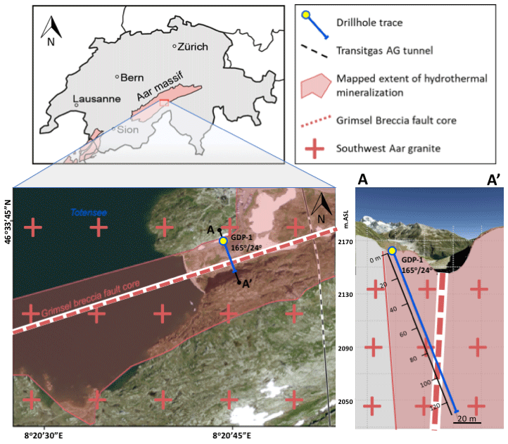
Figure 1Lower left shows an aerial image (source: Federal Office of Topography, https://www.swisstopo.ch, last access: 10 February 2017) of the Grimsel Pass showing the trace of the GDP1 borehole, the extent of mineralized outcrops associated with the GBF (Belgrano et al., 2016), and the location of the Transitgas AG tunnel with the interval of active hydrothermal inflow marked by the white stippled line (modified from Egli et al., 2018). The lower right shows a schematic cross section through the plane of the borehole intersecting the GBF showing the extreme topographic relief in conjunction with the location and orientation of the borehole (modified from Greenwood et al., 2019).
A list of all geophysical borehole datasets collected along the GDP1 borehole during 2015, 2016, and 2017 is shown in Table 1 together with the respective condition of the borehole at the time of their acquisition. Throughout this paper, all data are referred to and displayed with regard to measured depth along the borehole track. The most complete dataset was collected in 2015 directly after drilling under open borehole conditions. It comprises OTV, borehole caliper, passive and active nuclear, electrical resistivity, SP, temperature, and multiple center frequency FWS logs as well as constant offset BHR, ambient (and pumped) flow meter, and periodic pumping test measurements.
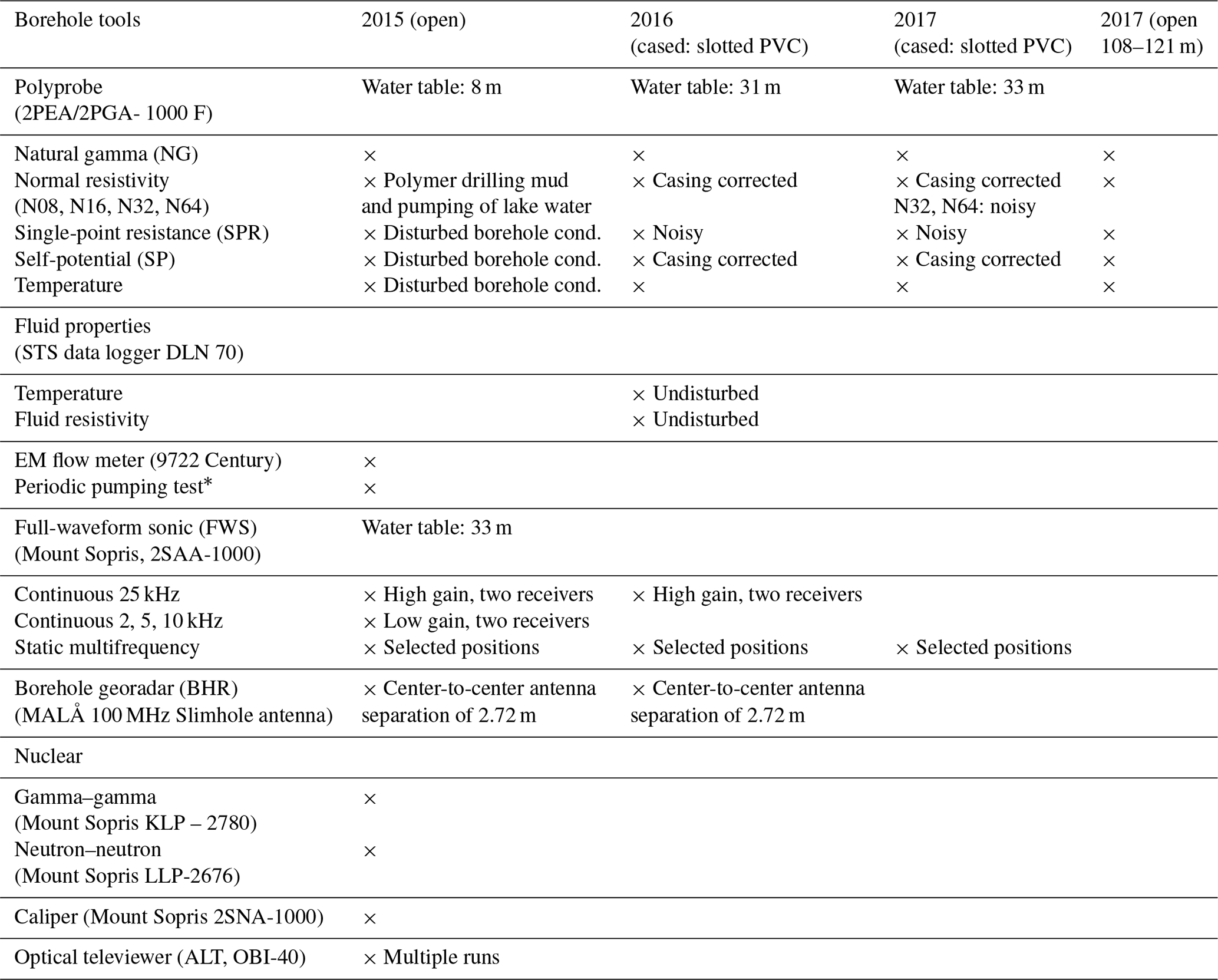
After completion of the drilling operations, water from the adjacent lake was pumped into the borehole to flush out the polymer-based drilling mud and to enable OTV measurements. Although, the water in the borehole cleared up, remnants of the drilling fluid within the adjacent formation were likely to be present throughout the 2015 logging campaign. As a consequence, the SP data acquired in 2015 differ significantly from those measured in 2016 and 2017 since the polymer-based drilling mud changed the viscosity and the chemical composition of the pore fluid in the rock volume with regard to its ambient state. In addition to this, the 2015 SP data were also affected by changes in the flow regime in and around the borehole induced by the pumping of lake water. In the following, we therefore only consider the SP data acquired in 2016 and 2017. The addition of the lake water and the remnant presence of drilling mud also affected the 2015 electrical resistivity measurements. These were therefore repeated in 2016 and 2017 through the slotted PVC casing, which was installed to prevent borehole collapse. To analyze the effects of this casing as well as for data calibration purposes, a small section at the bottom of the borehole was remeasured under open borehole conditions in 2017. Details with regard to the data corrections applied to remove the casing effects are given in Appendix B and Toschini (2018). EM flow meter tests, recorded in 2015, are also affected by the severely disturbed flow system as well as the fact that the polymer drilling mud potentially kept clogging some of the flow paths. Thus, only the passive data will be shown here for completeness of information.
BHR measurements were repeated in 2016, as no zero-time correction was available for the data collected in 2015. However, the 2015 data were acquired with a smaller spatial sampling interval and thus produce more coherent signals. For this reason, we utilize the 2016 data for calibration of the 2015 dataset, which we then consider for the remainder of the paper. Corresponding details are given in Appendix A. Additionally, more detailed temperature and fluid resistivity measurements were conducted in 2016. High-frequency (25 kHz nominal center frequency), high-gain three-receiver FWS data were acquired in 2016 for more reliable and robust compressional (P) and shear (S) wave velocity estimations by semblance analysis (Hornby, 1989). In the intensely fractured zones, especially around the main fault core, the first arrivals are, however, still very weak, thus making reliable velocity estimations very difficult due to the inherent uncertainty and local variability in the picks. Therefore, the P-wave velocity estimates are smoothed, and the S-wave velocity is entirely discarded in this zone. Everywhere else, the P- and S-wave estimates are reasonably robust.
Overall, the logging data are affected by strong borehole enlargements, which complicates their quantitative analysis. The enlargements are primarily due to the intensely fractured nature of the rock volume rather than being purely drilling-induced damage. Most of the enlargements can indeed be associated with distinct fractures or cataclastic features along the borehole track and thus present structural and petrophysical indicators in their own right. Geochemically the rock mass of the damage zone surrounding the GBF core is relatively homogeneous consisting of metagranite. The main heterogeneities are variations in fabric, ranging from granitic through gneissic, all the way to mylonitic as well as fractured and cataclastic zones, which are due to different degrees of ductile and/or brittle deformation (Egli et al., 2018). In the following, we seek to link these geological features inferred from the OTV and core data to the responses of the geophysical borehole logs. In a first step, we utilize the BHR data to image the fracture network situated in the damage zone. Then, the response of selected borehole log data is compared to different degrees of deformation encountered.
In contrast to most other geophysical borehole logging techniques, which have a relatively limited range of investigation, the BHR reflection method allows one to image individual fractures, clusters of fractures, and cataclastic zones outside of the immediate vicinity of the borehole (e.g., Olsson et al., 1992; Dorn et al., 2012). As such, these data are much less affected by borehole enlargements than most other logging data. In the considered setting, the reflection coefficient is governed by the pronounced contrast of the dielectric permittivity between the host rock and the fluid-filled fractures, while the bulk electrical conductivity of the rock volume determines the attenuation of the BHR signals. This, in turn, makes resistive crystalline environments ideal sites for BHR measurements in general and for imaging fractures in particular. In the following, we first describe the processing of the BHR data and then proceed to analyze the migrated images.
3.1 Data processing
Steeply dipping reflections are already visible in the raw data (Fig. 2a). To extract these reflections, the direct wave is removed via an alpha-trimmed 2D spatial filter after applying a static correction to flatten out the first arrivals. Subsequently, this static correction is reversed to place the reflections back into their original position (Fig. 2b). Since, the dataset was acquired with omnidirectional antennae, we can only determine the relative dip of the reflectors with respect to the borehole trajectory. It is not possible to constrain the azimuthal orientation of the reflectors. However, the OTV data indicate that the azimuths of most brittle and ductile structural features are constrained to one quadrant (Fig. 2c). Hence, it is justified to treat the reflections as up- and down-going wavefields originating at the same reflectors. Correspondingly, these up- and down-going wavefields are separated by f-k quadrant filters, then migrated using pre-stack Kirchhoff time-migration and converted to distance using a constant average velocity. Since the prevailing geological structure is near-vertical, the velocity is varying laterally, which was at least partially accounted for in the pre-stack time-migration process by a laterally varying velocity model derived from the first arrivals. Pertinent details of the processing and imaging flow applied to the BHR reflection data are given in Table 2.
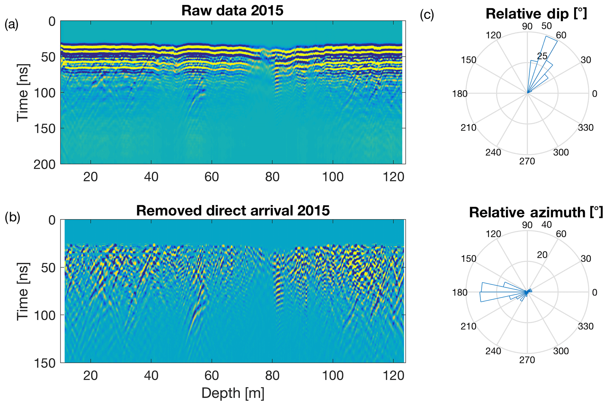
Figure 2(a) Raw BHR reflection data and (b) after removal of the direct wave and reversed static corrections. (c) Relative dips and azimuths of fractures identified in the OTV data.

3.2 Estimation of fracture dip
Figure 3a shows the final migrated and distance-converted BHR reflection image, which consists of the up- and down-going wavefields, plotted in positive distance orthogonally from the borehole trajectory. We observe an abundance of reflections, most of which intercept the borehole wall. It is straightforward to calculate the relative dip of these events. In zones of low attenuation, which correspond to large first-cycle amplitudes of the direct wave in Fig. 3b, some of these events can be traced to distances of up to 10 m from the borehole. These zones are representative of more intact rock. Conversely, high signal attenuation, characterized by low first-cycle amplitudes in Fig. 3c, occurs in zones of intense brittle deformation, such as, for example, in the fault core and its vicinity.

Figure 3(a) Migrated BHR image consisting of the up- and down-going reflection data plotted in positive distance from the borehole trajectory. Red lines denote selected reflection events used for estimating the dips and locations of the associated fractures. (b) Maximum first-cycle amplitude of BHR first arrivals (black line), relative dip of fractures from OTV data (turquoise dots), and relative dips picked from the depth-converted BHR reflection image (red dots and squares). For the OTV data, the size of the dots is a relative measure of fracture aperture. The dips of events denoted by red lines in (a) are identified by red dots encircled in blue.
From the image shown in Fig. 3a, we manually pick the dips of the brightest reflections as well as some of the weaker cross-cutting events to capture the variety of dips encountered. A representative selection of the picked events is superimposed on the image as straight red lines, and their locations with regard to the borehole track and their dips are illustrated in Fig. 3b by red dots encircled in blue. All picked events are plotted in Fig. 3b, and their values are compared to the fracture dips inferred from the OTV data, which are shown as turquoise dots whose diameter is indicative of the fracture aperture (Egli et al., 2018). Following Egli et al. (2018), fractures with very large apertures are classified as cataclastic zones; aperture refers here to the thickness of the fractures and not to the mean open space. Most of the fractures with a large aperture contain some infill. Overall, the range of dip angles picked from the imaged BHR reflection data is consistent with those inferred from the OTV data, although it is difficult to match individual reflection events with specific fractures in the OTV images. The reason for this is 2-fold. (1) Both datasets contain the signatures of an abundance of fractures, which, in turn, necessitates an inherently subjective selection; and (2) the depth locations and dips assigned to BHR reflectors might differ slightly with regard to those of the OTV data.
Nevertheless, the comparison of the two datasets confirms that in such an environment fluid-filled fractures and cataclastic zones are the most likely cause of BHR reflections. The BHR reflection image allows one to trace the associated brittle deformation structures several meters from the borehole into the adjacent formation. The BHR reflection image and the OTV data provide clear and consistent evidence for a dense and complex network of fluid-filled intersecting fractures and cataclastic zones above and below the main fault core. Such a network of fractures provides effective fluid pathways through the otherwise tight granitic host rock (e.g., Berkowitz, 2002).
4.1 Full-waveform sonic data: identification of brittle deformation zones
As illustrated by Fig. 3b, the first-cycle amplitude of the BHR first arrivals is a good proxy for the degree of brittle deformation. Similarly, FWS data are expected to be sensitive to brittle deformation as the associated wave propagation is governed by the underlying elastic and hydraulic properties of the medium. Here, we utilize the 2 kHz low-gain FWS data, which are mainly sensitive to low-frequency Stoneley waves. This wave type is an interface wave traveling along the borehole wall. Its velocity depends predominately on the shear modulus of the formation and bulk modulus of the fluid. Its amplitude decreases across compliant and hydraulically transmissive features, such as fractures and cataclastic zones, due to transmission losses, reflections, and pressure diffusion processes (e.g., Paillet, 1994). Following Paillet (1983), the local Stoneley wave energy deficit can be used as an indicator of the hydraulic transmissivity of a system. For the considered data, a quantitative analysis is, however, not possible, since the data quality due to the roughness of the borehole wall caused by enlargements as well as the recording time are not sufficient, and the data recorded at receiver 1 is clipped even for the lowest possible gain of the tool. Nevertheless, we can still estimate the local energy deficit of the recorded waveforms, which are dominated by Stoneley waves, and use this measure as a qualitative proxy. To account for borehole enlargements, we compare the FWS data with the caliper and the neutron–neutron log data. While the neutron–neutron log is also affected by the borehole enlargements, it is primarily sensitive to the water content and thus to the porosity, which in the considered environment is dominated by fracture porosity (Egli et al., 2018).
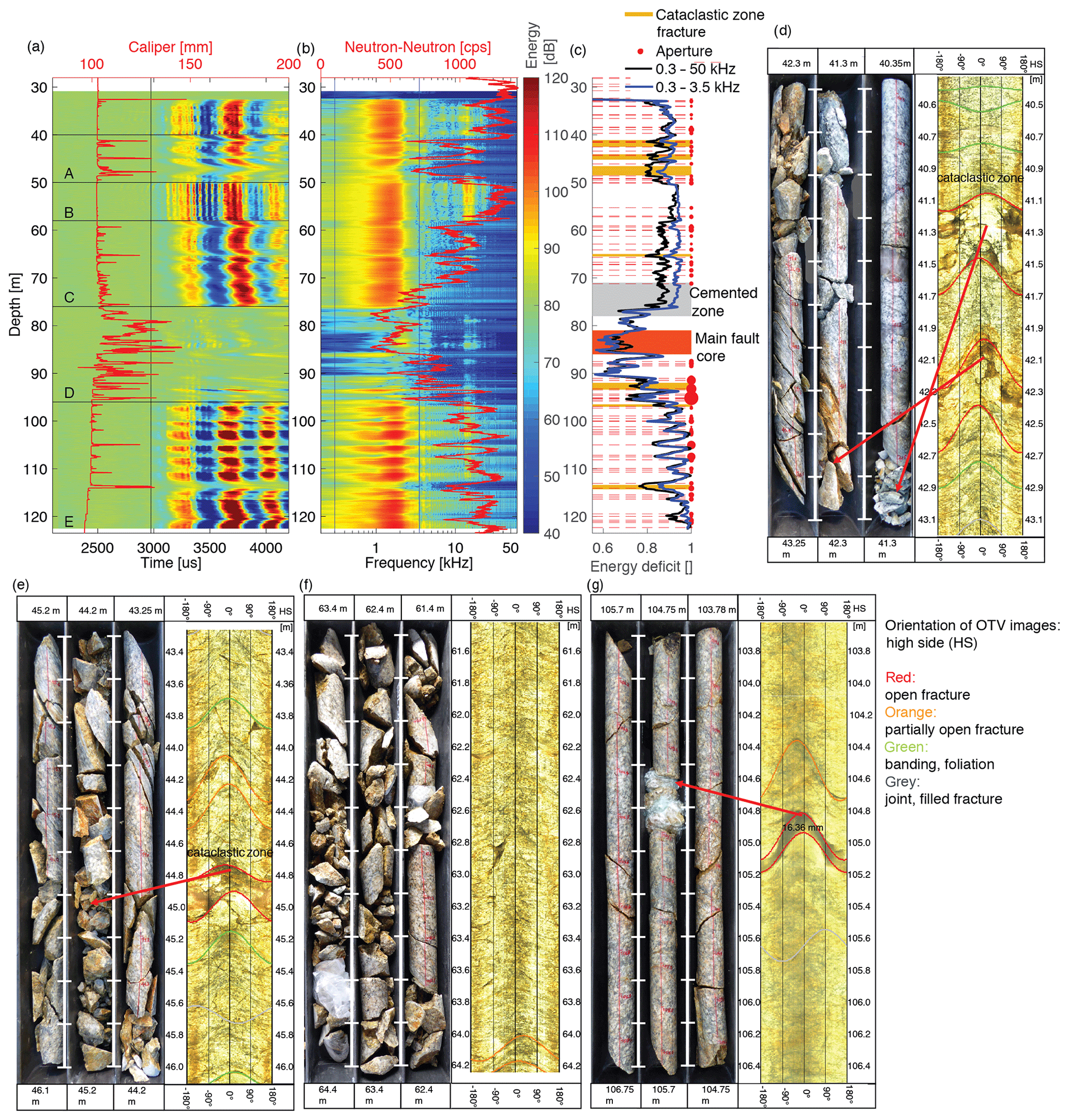
Figure 4(a) Low-gain FWS data acquired with a nominal central frequency of 2 kHz overlain by the caliper log; (b) corresponding power spectrum overlain by the neutron–neutron log; (c) relative energy deficit for two different frequency bands, one capturing the Stoneley wave and the other the complete spectrum, in conjunction with the first-cycle amplitude of the BHR direct wave and the brittle deformation data from the OTV; (d–g) examples of brittle deformation based on a comparison of OTV data and corresponding drill core sequences.
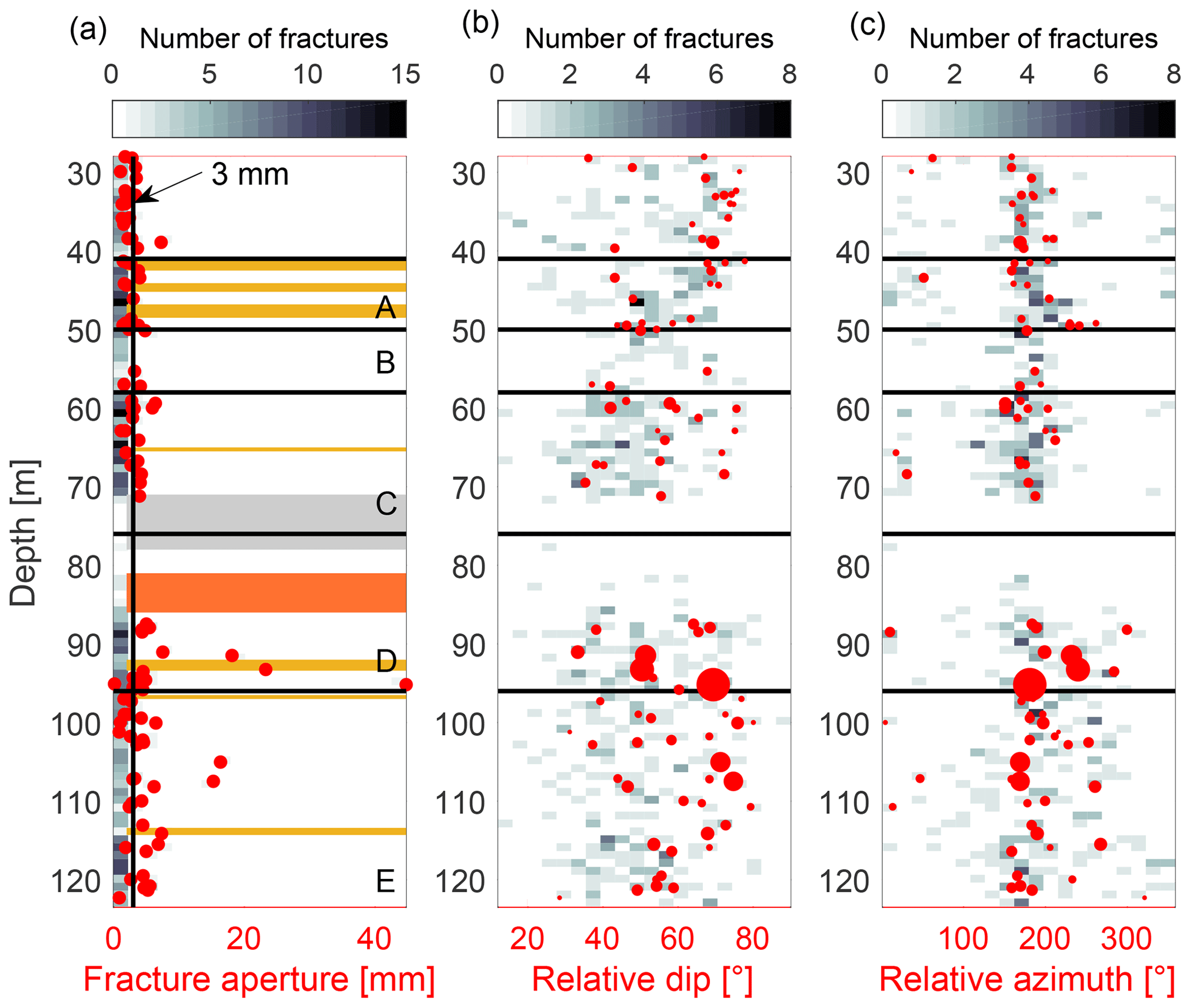
Figure 5Summary of the brittle deformation based on the OTV data (Egli et al., 2018) (a) fracture aperture, (b) relative dip, and (c) relative azimuth. All identified fractures are displayed in histographic form along the borehole. Fractures with measurable aperture (greater than 0.8 mm) are displayed as red dots. In (a) additionally cataclastic zones, the cementation zone, and main fault core are plotted.
In Fig. 4, we compare the aforementioned log data to the OTV-based brittle deformation data of Egli et al. (2018). Figure 4a shows the low-gain FWS log data recorded at receiver 2 for a nominal center frequency of 2 kHz and Fig. 4b the corresponding power spectrum. The former is overlain by the caliper log and the latter by the neutron–neutron log. The color scale in Fig. 4a is chosen such that the primarily visible signal is the Stoneley wave. The first arrival P- and S-waves are much lower in amplitude. The local energy deficit is shown in Fig. 4c for two frequency bands and overlain with the OTV-based brittle deformation data of Egli et al. (2018). Figure 4c also depicts the BHR first-cycle amplitude. From the FWS data, we can clearly distinguish five characteristic zones denoted as A through E, which also find their expressions in the first-cycle BHR amplitudes. In the following, we compare these zones to the brittle deformation data of Egli et al. (2018), which is summarized in Fig. 5, comprising the apertures as well as the relative dip and azimuth of the fractures with respect to the horizontal of the borehole trajectory. Apertures below 0.8 mm were deemed not to be reliably measurable for the recorded resolution of the OTV data.
-
Zone A consists of three cataclastic zones. The OTV image and the core material of two cataclastic zones are shown in Fig. 4d and e. These cataclastic zones are characterized by time-delayed, low-amplitude Stoneley waves with an energy reduction of 15 % as well as low BHR amplitudes. Moreover, they find their expression as prominent anomalies in the caliper and neutron–neutron logs. As such, zone A is likely to represent a hydraulically transmissive interval of low shear strength and high porosity.
-
Compared to zone A, zone B is characterized by a smaller energy deficit and an overriding high-frequency wave corresponding to the pseudo-Rayleigh wave, which only exists in fast formations and thus suggests a zone of higher shear strength and less brittle deformation. The latter is consistent with the high BHR amplitudes. Nevertheless, even in this section, fractures are still present (Fig. 5), albeit with apertures below 0.8 mm.
-
Conversely, the FWS signal in zone C is dominated by low frequencies in the power spectrum with a decrease in high frequencies towards zone D and the vanishing of the pseudo-Rayleigh wave, which is indicative of a decrease in shear strength. The BHR amplitudes decrease towards zone D as well, in which the borehole collapsed and had to be cemented and redrilled. The BHR amplitudes already show a strong decrease at 70 m depth, whereas the other logs (caliper, neutron–neutron, energy deficit) only show a pronounced changes around 75 m. Due to their small penetration depths, the latter are affected by the cemented section of the borehole, whereas the BHR measurements have a deeper penetration depth and are averaged over a larger support volume. Thus, the BHR measurements are likely to reflect the “true” formation properties better in this section. The core material in zone C (e.g., Fig. 4f) is partly noncohesive due to intense brittle deformation, which explains the observed characteristics of the BHR amplitude and FWS data. Local vanishing of the FWS amplitudes in conjunction with anomalies in the caliper and neutron–neutron logs at 65 to 65.3 and 66.74 m are due to a cataclastic zone and an individual large-aperture fracture of 3.71 mm, respectively.
-
Zone D comprises the wider zone of the main fault core where most of the FWS signal is lost. One reason is the large borehole enlargements and the associated rugosity of the borehole wall, which prevents the propagation of Stoneley waves. In the upper part of this zone, a weak signal is recorded between a borehole depth of 82 and 86 m with a shift towards higher frequencies. This section corresponds to the GBF core consisting of fault gouge (Egli et al., 2018).
-
Finally, zone E is characterized by an alternating sequence of regions with pronounced low and high energy deficits, which is indicative of an overall rather compact rock volume with prominent isolated fractures (e.g., Fig. 4g). This interpretation is consistent with a correspondingly alternating sequence in the BHR amplitudes.
4.2 Cluster analysis
To refine the zonation identified in Fig. 4 and infer the associated petrophysical properties, we consider a pertinent selection of the logging data acquired in 2015 under open-hole conditions and in 2016 through a screened PVC casing. These are shown in Fig. 6 and include from left to right the caliper and natural gamma log, the sonic P- and S-wave velocities, the gamma–gamma and neutron–neutron logs, the BHR direct-wave velocity and amplitude, and electrical resistivity measurements. All logs are superimposed onto the brittle deformation data mapped from the OTV. The larger-scale trends of most of the logs are consistent with the previously inferred zonation A through E, which is depicted on the left-hand side of Fig. 6. The GBF fault core, which is located between 82 and 86 m borehole depth, is marked by borehole enlargements and clearly defined across the entire suite of logs. Most of the remaining anomalies observed in the borehole log data correlate with caliper anomalies, which, in turn, are associated with enlargements and can be linked to zones of the brittle deformation identified in the OTV data. In the following, we analyze the relationship between the various borehole logs and address the question whether their response can be linked to the degree of brittle deformation. To this end, we perform a cluster analysis on a selection of the log data.
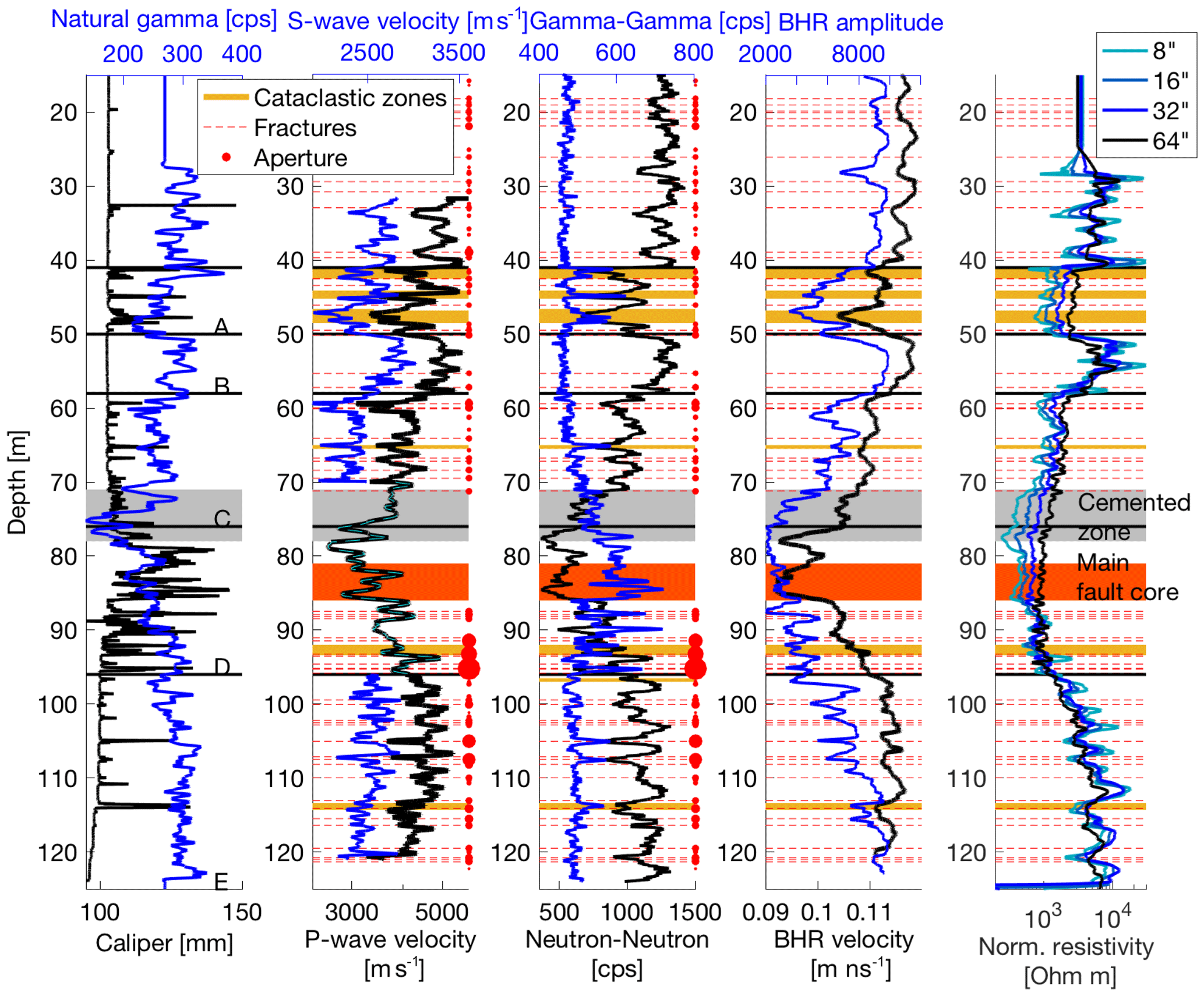
Figure 6Representative selection of borehole log data comprising from left to right caliper, natural gamma, sonic velocity, neutron–neutron and gamma–gamma, BHR direct-wave velocity, and amplitude as well as normal resistivity logs with a separation of 8 in. (0.2 m), 16 in. (0.4 m), 32 in. (0.8 m), and 64 in. (1.6 m). The brittle deformation features interpreted from the OTV data (Egli et al., 2018) are superimposed on the log data. The sizes of the circles are indicative of the relative fracture apertures. Zones A through E refer to zonation shown in Fig. 4.
In a first step, we perform a correlation analysis of the log data shown in Fig. 6. Before doing so, the datasets are normalized to account for the different unit scales. We obtain an overall good correlation between the BHR velocity and amplitude and the neutron–neutron, the P-wave velocity, and the normal resistivity logs. In the following, these datasets will be subjected to a cluster analysis. Although the S-wave velocity log shows a good correlation with other log data in the more intact parts of the borehole, it is not considered due to its unreliability around the main fault core. The gamma–gamma log is strongly affected by large borehole enlargements and shows otherwise little variation. The poor correlation of the natural gamma log with the other datasets is probably due to the fact that, in the crystalline environment, it is primarily sensitive to mineralogical alterations, which, compared to the brittle deformation structures, have a secondary effect on the other borehole logs. The BHR velocities and amplitudes are primarily sensitive to the fluid-filled porosity and the bulk electrical conductivity, respectively. The neutron–neutron log is sensitive to the total amount of hydrogen present in the formation, while the P-wave velocity log is sensitive to the mechanical properties, and the normal resistivity is sensitive to the bulk resistivity.
The upper triangular region in Fig. 7 shows crossplots of the selected log data, which confirm the overall good correlation. The somewhat spurious nature of these crossplots is due to the fact that the various geophysical logs average the petrophysical properties over significantly differing support volumes. This is problematic when dealing with small-scale, high-contrast features, such as fractures, embedded in an otherwise relatively homogeneous matrix. An effective way to display such datasets is in histograms, as shown in the triangular region below the diagonal in Fig. 7, which clearly illustrate the overall strong correlation trends between the various datasets. The largest spread of values is observed for crossplots containing either the P-wave velocities or the BHR amplitudes, whereas the other properties show generally well-defined correlation trends.
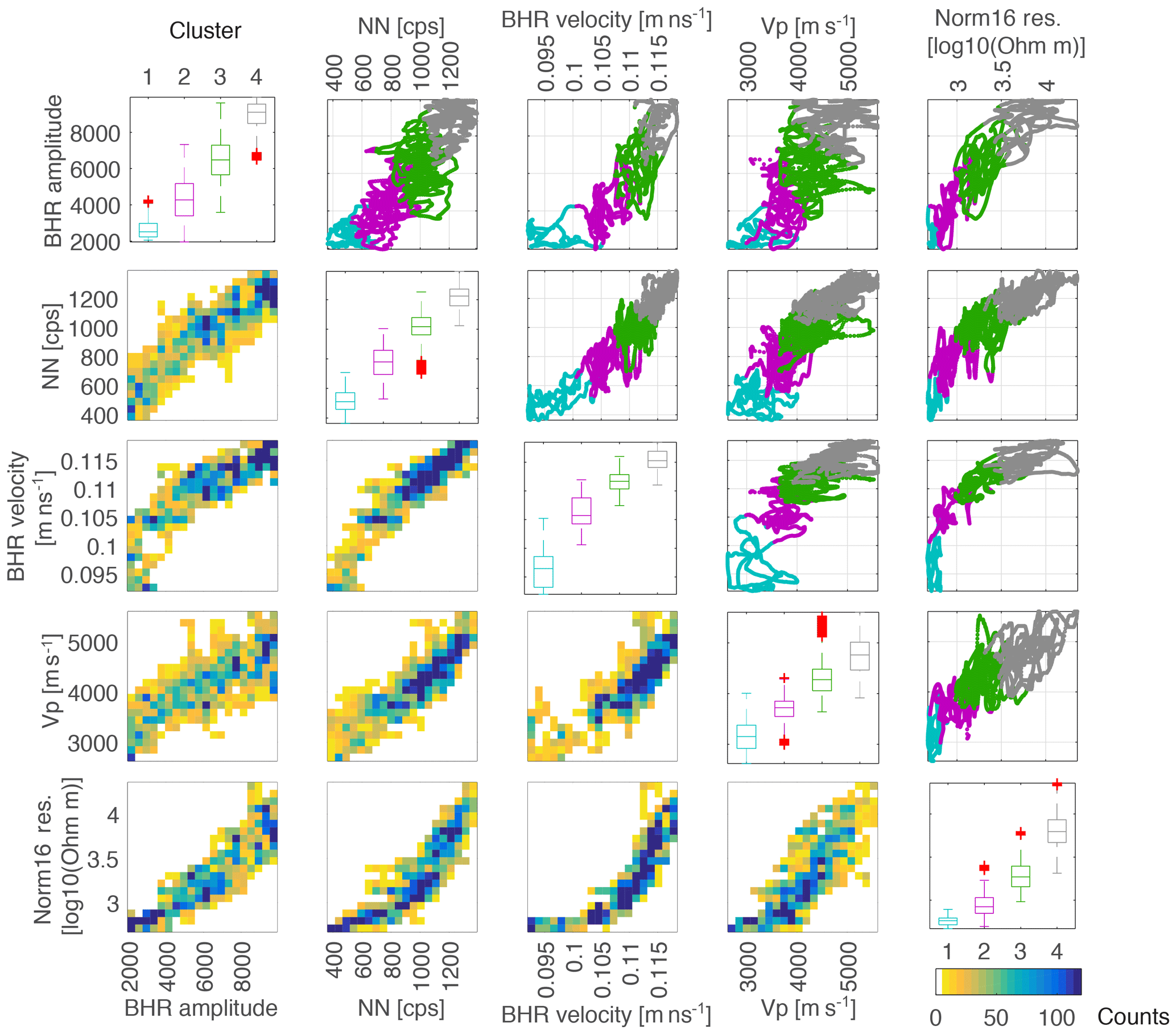
Figure 7Lower triangle with regard to diagonal: histogram crossplots of selected borehole logs – BHR amplitude, neutron–neutron (NN), BHR velocity, P-wave velocity (Vp), and normal resistivity 16 in. (0.4 m) (Norm16 res.). Upper triangle with regard to diagonal: color-coded crossplots of groups identified based on cluster analysis. The diagonal shows the corresponding cluster boxplots for each property.
To analyze these trends in more detail, we perform a cluster analysis using the k-means algorithm of the MATLAB Statistics Toolbox with a squared Euclidian distance criterion (Arthur and Vassilvitskii, 2007). The analysis is performed on the normalized data in two subsequent steps. First, we test for the optimal number of clusters to group the data into. To do this, we use the so-called silhouette and gap criteria (Tibshirani et al., 2001), which both suggest an optimum of four clusters. Then, we apply the k-means algorithm to group the data into four clusters. The median, the 25th percentile, and the outliers of each cluster and each petrophysical property are shown in the form of boxplots along the diagonal of Fig. 7. Across all petrophysical properties, the identified clusters show a good separation with regard to each other.
Figure 8 shows the borehole log data used for the above cluster analysis color-coded according to the four cluster groups identified in Fig. 7 and overlain by OTV-based brittle deformation data. Also shown is the sequence of clusters along the borehole track together with the fracture density inferred from OTV data as well as the caliper log. Comparing these various datasets allows the characterization of the clusters as follows: (1) GBF fault core, (2) zones of high fracture density or cataclastic deformation, (3) zones of moderate fracture density or large-aperture fractures, and (4) zones of low fracture density. There is a mismatch at the bottom of the borehole between the cluster-based interpretation of the borehole log data and fracture density estimated from the OTV data. The reason is that partially and fully closed fractures are accounted for in the OTV-based fracture density, while the logs are largely insensitive to these types of fractures. This problem only manifests itself at the bottom of the borehole, since the occurrence of closed fractures compared to open fractures is larger in this region than elsewhere along the borehole. An essential result of the cluster analysis is that the signatures of the selected borehole logs as well as their interrelations are predominantly governed by brittle deformation in general and that the individual clusters seem to be clearly linked to the degree of deformation in particular. In this context, it is interesting to note that the sequence of clusters along the borehole displayed on the righthand side of Fig. 8 is fully consistent with the more generic zonation A through E inferred from the Stoneley wave analysis (Fig. 4).
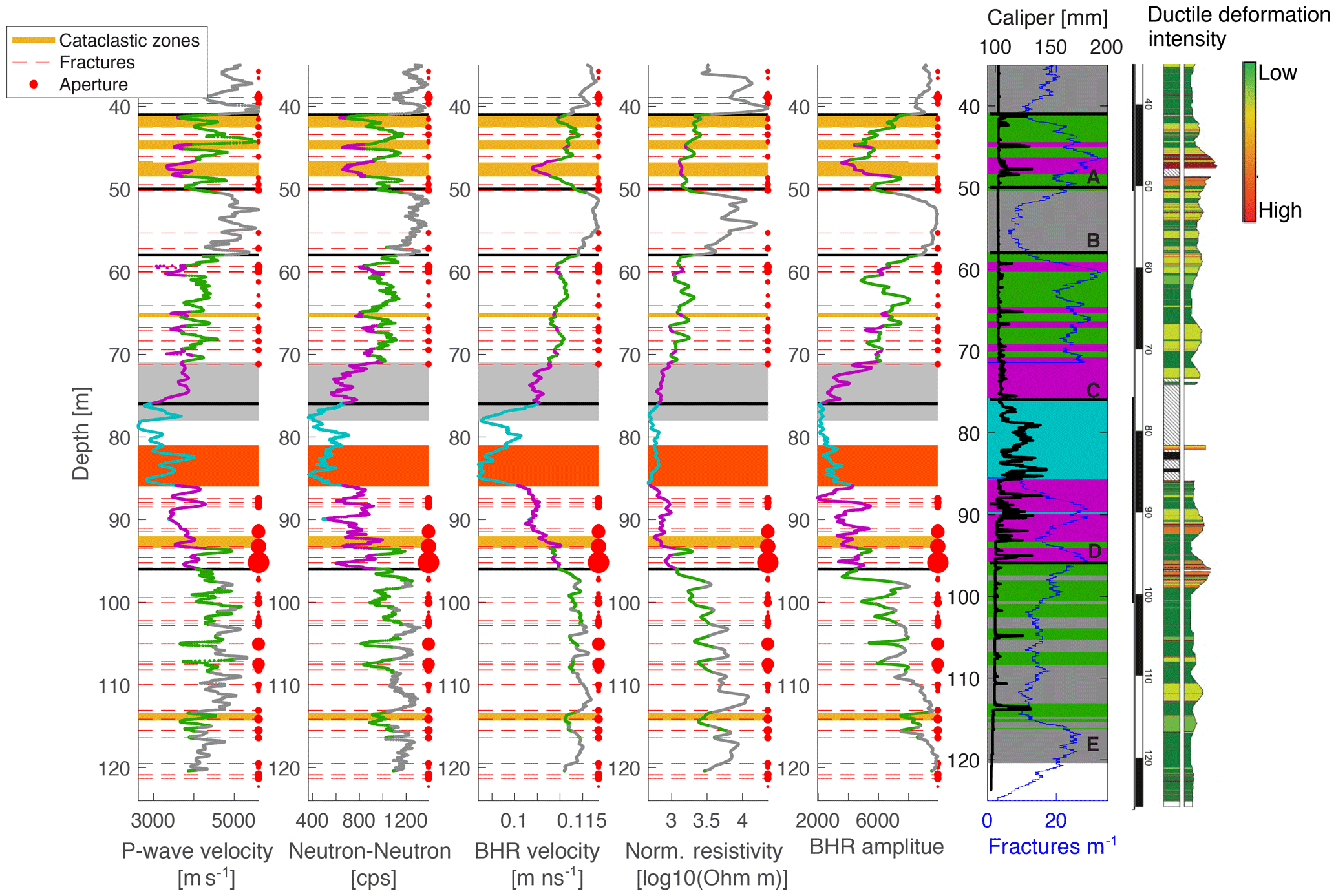
Figure 8Borehole log data used for cluster analysis, color-coded according to the four cluster groups identified in Fig. 7 and overlain by brittle deformation inferred from the OTV data. The righthand column shows the sequence of clusters along the borehole together with the fracture density inferred from the OTV data, the ductile deformation intensity log (Egli et al., 2018), the caliper data, and the zonation A through E inferred from the Stoneley wave analysis (Fig. 4).
Interestingly, the P-wave velocities and normal resistivity data exhibit a larger variability in cluster 4 than in the other petrophysical properties. This becomes especially apparent in zone B, which exhibits a comparatively low fracture density and variable degrees of ductile deformation (Fig. 8). In this partially intact zone, the P-wave velocity assumes maximum and minimum values of 5600 and 4600 m s−1, respectively. The former is close to P-wave velocities of non-fractured granitic rocks, which typically range between 5700 and 6200 m s−1 (e.g., Holbrook et al., 1992; Salisbury et al., 2003). The variability in the P-wave in these more intact zones might thus be an indication of variations in the ductile rock fabric. We also observe strong fluctuations in electrical resistivity and relatively low resistivity values on average for a granitic environment. The latter may point towards the influence of surface conductivity, most likely due to the abundance of mica notably in the gneissic and mylonitic parts of the formation, which, in turn, may result in regions of elevated conductivity compared to the unaltered granites (Keys and Sullivan, 1979). A recent study of electrical properties of mylonites from the Alpine Fault project in New Zealand found resistivity values ranging from 675 to 75 Ω m (Kluge et al., 2017). This is significantly lower than literature values of granite, which range from 103 to 106 Ω m. The variability in the P-wave velocity and resistivity is also reflected in the natural gamma log, which, in turn, points to the potential influence of mineralogical changes associated with ductile deformation.
Although the borehole logging data are clearly related to the degree of fracturing, which is expected to be a proxy for fluid flow, a quantitative analysis in terms of key hydraulic properties, such as porosity and permeability, in the studied environment is challenging. The reasons are manyfold. As previously mentioned, the Stoneley wave data are not of sufficient quality to allow for corresponding permeability estimations. The gamma–gamma and neutron–neutron logs, which are classically used to determine the porosity via the density and the hydrogen content, respectively, are affected by the large variations in the borehole diameter. These enlargements make a calibration of the gamma–gamma log to obtain density and subsequently porosity essentially impossible. The neutron–neutron log is less affected by the caliper variations than the gamma–gamma log, but calibrating it is still difficult due to its nonlinear relation to the hydrogen content and the lack of representative core material over a large enough porosity range. The resistivity logs, cannot not be converted into porosity, since the fluid resistivity is very high compared to common groundwater, the matrix porosity is quite low, and the surface conductivity can possibly not be ignored, which renders Archie's law inapplicable (e.g., Glover, 2015). This is illustrated in Appendix A by comparing the resistivity logs with Archie's law. To circumvent these problems associated with the commonly used porosity logs, we use the 2015 BHR velocity measurements to derive porosity estimates. BHR measurements are not commonly utilized in oil and geothermal reservoirs, but there use is quite common in groundwater investigations to estimate water content or equivalently porosity (e.g., Bradford et al., 2009). The approach is quite robust, since the method is strongly sensitive to the water content and has a large support volume, which makes it less susceptible to borehole enlargements. The resulting smooth porosity profile will be then used to calibrate the neutron–neutron log, which provides a detailed downscaled version of the porosity distribution along the borehole. In a subsequent step, we examine the fluid flow characteristics of the subsurface region based on a combined analysis of the SP, temperature, and resistivity logs.
5.1 Porosity estimation
The porosity ϕ is obtained from the BHR velocity v using the so-called complex refractive index method (CRIM)
where c is the speed of light and v the velocity of the formation; ϵr, ϵw, and ϵs are the relative dielectric permittivities of the formation, the pore water, and the solid material, respectively (e.g., Greaves et al., 1996). For low porosities, the method is quite sensitive to the dielectric permittivity of the solid material ϵs. To find a representative value for ϵs, we constrain the possible range by laboratory-based density measurements. Archimedes-type density measurements have been performed along the entire core recovered from the GDP1 borehole. These measurements were taken at 20 to 30 cm intervals (Jörg Renner, personal communication, 2016). The inferred densities are compared to densities calculated from BHR porosities for different values of ϵs (Fig. 9a) using an average grain density of 2653 kg m−3 determined from corresponding laboratory analysis of eight samples measured. Subsequently, an upper and lower bound for ϵs is chosen so that the laboratory-measured densities from competent samples fall between the resulting calculated density values from the BHR velocities. This provides well-constrained bounds for low and intermediate porosities. However, the estimation of high porosities is less reliable due to core loss and poor quality of the retrieved core material from the heavily fractured zones. The results are shown in Fig. 9b together with the porosity curve for the median of the best-fitting dielectric permittivity. For the latter, we only consider the zones without borehole enlargements.
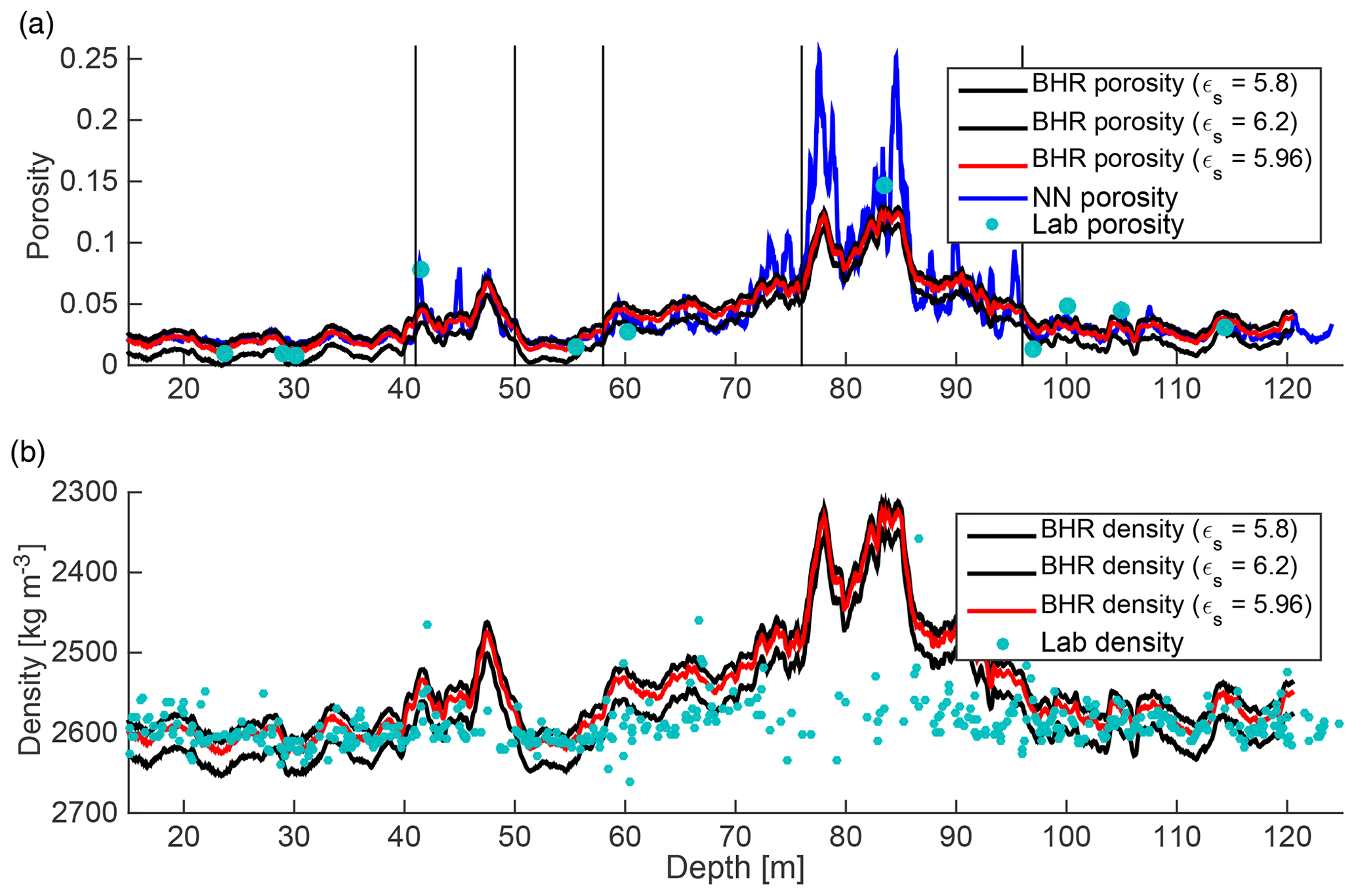
Figure 9(a) Porosity estimates from BHR velocities for different dielectric permittivities of the solid material ϵs and from neutron–neutron (NN) data compared with laboratory-based measurements for selected core samples (Jörg Renner, personal communication, 2016). (b) Inferred density from BHR porosities compared to Archimedes-type density measurements on the core samples (Jörg Renner, personal communication, 2016).
The resulting porosity logs obtained from the BHR velocity measurements are, as expected, smooth due to the large support volume of the method, and, hence, the strong fluctuations in response to the intense fracturing observed in other borehole logs are averaged out. To capture the variability in the porosity on a smaller scale, the neutron–neutron measurements are utilized to downscale the BHR porosity. Details are given in Appendix A. The resulting downscaled porosity log is compared to laboratory-measured porosities for selected core samples (Fig. 9) and to a multiscale porosity analysis of Egli et al. (2018), which includes OTV data, thin sections, and He-pycnometry (Fig. 10a). Across all these different methods, the corresponding porosity estimates agree remarkably well. Figure 10b shows the sequence of brittle deformation groups inferred from the cluster analysis for comparison along the borehole. The largest porosities prevail, as expected, in the main fault core with a decreasing trend away from this zone. Other high-porosity zones are associated with cataclastic zones and large aperture fractures. Even in the most intact zones, the porosity is, however, still higher than common values of the matrix porosity in crystalline rocks of ∼1 % or less (Schmitt et al., 2003).
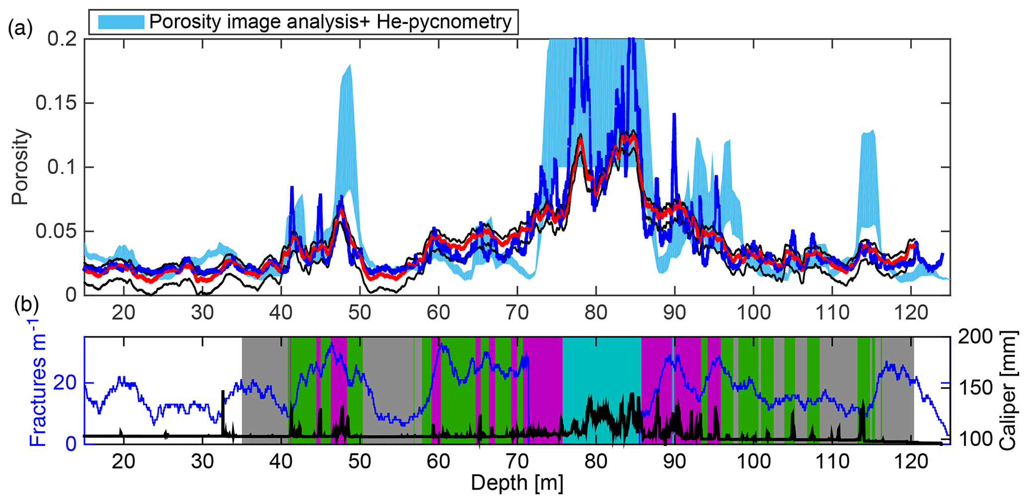
Figure 10(a) Comparison of log-based porosity estimates with corresponding values from thin section image analysis and He-pycnometry (Egli et al., 2018) and (b) brittle deformation groups inferred from cluster analysis (Figs. 7 and 8) with the caliper log and OTV-based fracture density log superimposed.
5.2 Fluid flow characteristics
The prevailing fracture network and high-porosity zones associated with brittle deformation are the main flow pathways of the GBF system in its present state. To shed more light on the hydraulic characteristics of this system, we analyze a combination of SP logs from 2016 and 2017 in conjunction with temperature and fluid resistivity logs. The first part of this subsection describes the processing and interpretation of the SP data, while the second part focuses on the combined interpretation of the various log data with respect to the fluid flow characteristics.
Self-potential data
The SP logs were acquired in the same logging run as the normal resistivity and single-point resistance logs. In this setup, the reference electrode for the SP measurements is the steel cable along which the logging tool is suspended. This causes a very strong drift in the measurements until ∼30 m of the exposed steel cable is below the water level; afterwards the measurements start to stabilize. For this reason, we only show measurements from 60 m borehole depth onwards for the 2016 and 2017 SP logs, as the water table was at 33 m borehole depth at the time of the measurements. To compensate for the remaining drift of the data, we removed a linear background trend (Appendix B). The resulting logs are shown in Fig. 11 and compared to the open-hole measurements at the bottom of the section acquired in 2017. There are some differences in the absolute values between the open- and cased-hole measurements, however, the main features of the data, especially the position and the character of the anomalies are the same. Overall, the anomalies in the SP logs along the entire considered depth range are pronounced and well defined and show remarkable repeatability between the data acquired in 2016 and 2017.
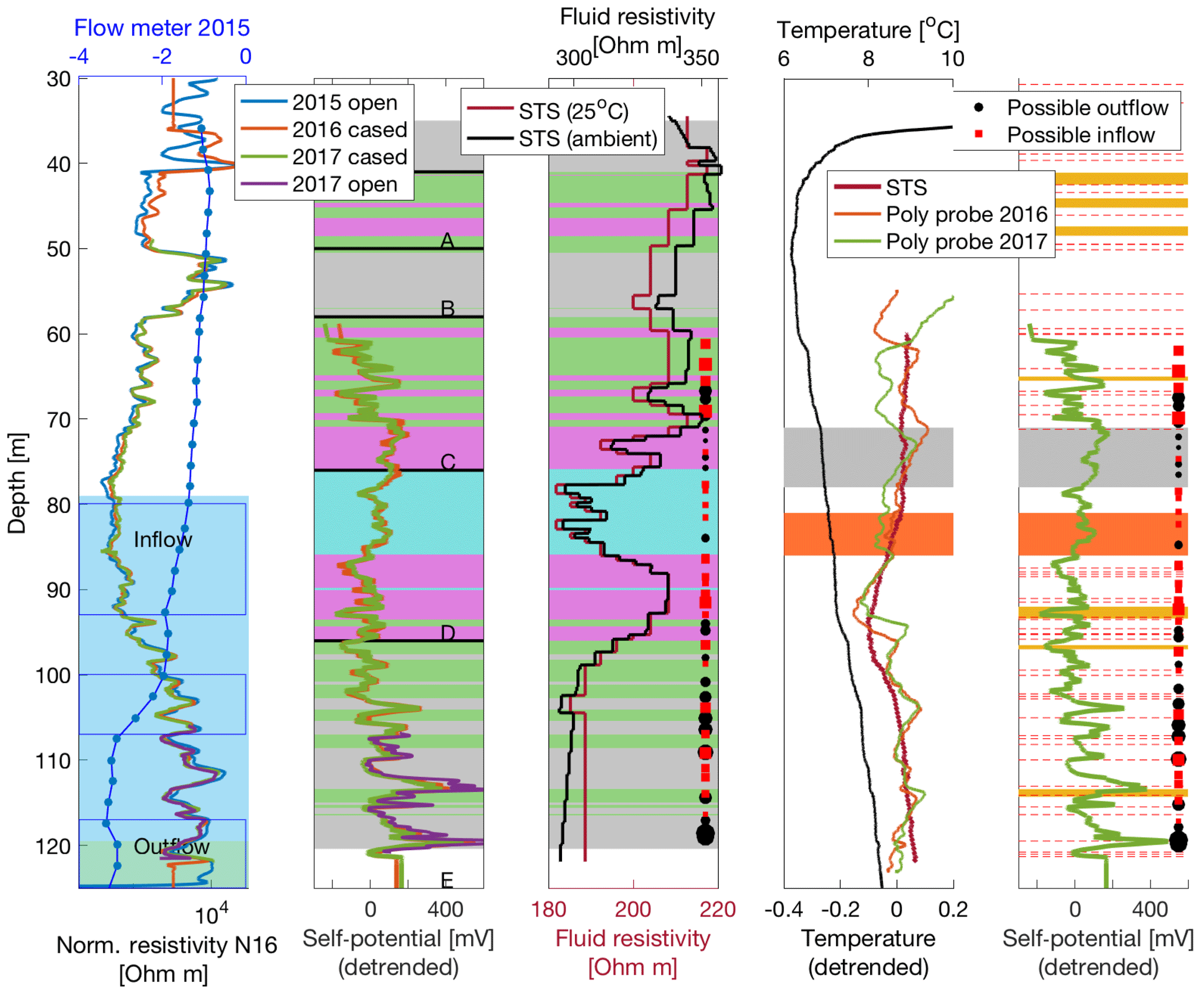
Figure 11Comparison of the trend-corrected SP data with complementary borehole logs. From left to right: electrical resistivity and zones of in- and outflow inferred from an analysis of natural hydraulic heads (Cheng and Renner, 2017) as well as passive flow meter tests (2015), results of cluster analysis (Figs. 7 and 8) overlain with the detrended SP data, the fluid resistivity log measured in 2016, the temperature logs, and the OTV-based brittle deformation logs (Egli et al., 2018) overlain by the SP data. The fluid resistivity measurements are shown at ambient conditions and corrected to a constant temperature of 25 ∘C. The detrended temperature logs of the polyprobe tool (2016, 2017) and the STS tool (2016) as well as the not trend-corrected temperature profile (black line) acquired with the STS (2016) tool are displayed.
SP anomalies can be of electrokinetic, electrochemical, and thermoelectric origin (e.g., Jackson, 2015). In the studied fractured hydrothermal environment, SP anomalies are most likely of electrokinetic origin. This assessment is supported by an analysis of flow meter data by Cheng and Renner (2017), which identified zones of in- and outflow into the borehole associated with hydraulically open fractures. For SP signals of electrokinetic origin, the corresponding streaming potential φ can be linked, to the first order, to the hydraulic pressure gradient Δp (e.g., Jackson, 2015)
where C<0 is the electrokinetic coupling coefficient. The magnitude of C depends on several factors. Notably, it scales with the electrical conductivity of the pore water over several orders of magnitude, thus justifying a simple empirical relation derived from laboratory data for estimating the coupling coefficient for field observations (Revil et al., 2003). Given that, at ambient conditions, the average fluid resistivity along the GDP1 borehole is ∼320 Ω m (Fig. 11), which is high compared to common groundwater, this results in a large coupling coefficient of mV MPa−1. This, in turn, can explain the large magnitudes of the observed SP anomalies, even in the presence of moderate to weak hydraulic pressure gradients. The high resistivity of the water in the borehole is not unusual for the area. The adjacent lake water, which has a direct glacial inflow and mostly consists of melt water, has a resistivity of ∼500 Ω m.
Figure 11 shows that the observed SP anomalies are abundant and reach values of up to 400 mV, which is indeed very large for signals of electrokinetic origin. Using the above estimate for the coupling coefficient of C ≈ −6600 mV MPa−1, the largest SP anomalies in our data, imply hydraulic pressure gradients on the order of 0.06 MPa. This is approximately one order of magnitude lower than the pressure gradients estimated by Suski et al. (2008) in a saline artesian fractured hydrothermal system for maximum SP anomalies of ∼50 mV. Despite their unusually large magnitudes for SP signals of electrokinetic origin, the anomalies observed along the GDP1 borehole thus seem to be realistic for the specific setting. Indeed, SP anomalies of similar magnitude were recorded in the Grimsel Test Site (Himmelsbach et al., 2003), which is situated in the same granitic formation ∼400 m below the Grimsel Pass. In this case, the anomalies could be attributed to electrokinetic responses of distinct fractures. An additional contribution to the measured SP signals along the GDP1 borehole could arise from variations in the bulk resistivity. This might come into play between 95 and 120 m borehole depth, where we observe relatively strong variations in resistivity, which are linked to the variable degree of fracturing, as illustrated by the results of the cluster analysis (Fig. 8).
Considering the described uncertainties and the abundance of SP anomalies due to the intensely fractured nature of the formation, associating a single anomaly deterministically with in- or outflow is impossible. To overcome this problem, we apply a probability tomography based on Di Maio and Patella (1994). This approach reconstructs an image of the most probable locations of SP sources, which explain the observed data by assuming that an anomaly measured at location can be represented by a linear superposition of partial SP effects due to elementary electric source elements located at . For the considered borehole measurements, we scan a region which cuts the borehole along its trajectory for such source elements with the scanning function
The result of this procedure is an electric charge occurrence probability (ECOP) map given by the cross-correlation between the scanning function and the electrical field associated with the SP measurements. For SP signals caused by a distribution of dipole sources, corresponding dipole occurrence probability (DOP) maps can be calculated for the horizontal and vertical component of the dipoles. A more detailed description of the method is given by Hämmann et al. (1997), Mauriello and Patella (1999), Iuliano et al. (2002), and Saracco et al. (2004).
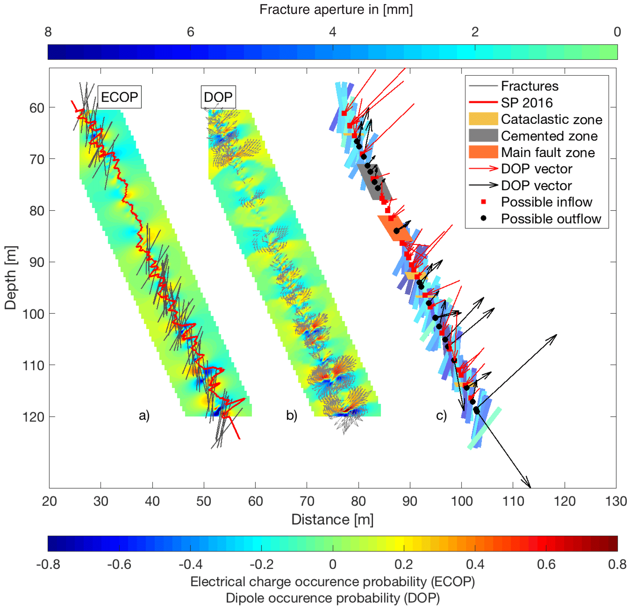
Figure 12(a) Electric charge occurrence probability (ECOP) and (b) dipole occurrence probability (DOP) maps along the borehole track overlain by the SP log and fractures from OTV data, and DOP vectors with an absolute probability larger than 0.15, respectively. (c) Most probable DOP vectors in each 1.2 m interval mapped onto the borehole track together with a projection of fracture planes and their color-coded apertures.
Figure 12a and b show the resulting ECOP and DOP for the largest of the two dipole components at each location along the borehole track. The DOP map is overlain by DOP vectors constructed from the horizontal and vertical dipole components. These vectors are indicative of the direction of fluid flow at a specific location. For display purposes, a threshold has been chosen, and only vectors with an absolute probability larger than 0.15 are shown. Also shown are the most probable vectors, which are selected in subsequent 1.2 m intervals and mapped onto the borehole trajectory together with the orientation and aperture of the fractures identified from the OTV data in Fig. 12c. Positive and negative values in the ECOP map indicate regions that gain and loose water, respectively; as such they are possible locations of in- and outflow along the borehole. The selected DOP vectors in Fig. 12c are color-coded correspondingly and indicate possible in- and outflow scenarios. For the interpretation of the hydraulic behavior, we focus on these scenarios.
5.3 Hydraulic zonation
The observed SP anomalies can be associated with fractures and cataclastic zones identified in the OTV data (Fig. 11). The representative DOP vectors and corresponding ECOP values indicate that above 95 m borehole depth inflow is dominating. Inflow into the borehole can be caused by flow from fractures and downflow along the borehole. Both scenarios are likely to occur. The former is supported by DOP vectors coinciding with the direction of the fracture dip suggesting flow along fractures and the latter by flow meter measurements conducted in 2015 indicating a generic downflow regime along the entire borehole (Fig. 11). Below ∼95 m borehole depth, the character of the SP data and the associated DOP vectors and ECOP values are more variable, including both inflow and outflow with an increase in the number of outflow regions towards the bottom of the borehole and a dominant outflow around 120 m borehole depth. These observations are generally consistent with results from flow meter measurements and an analysis of natural hydraulic heads by Cheng and Renner (2017). The study identified inflow between 81 and 119 m and a zone of prominent outflow below 119 m borehole depth, as indicated by the blue and green rectangles in Fig. 11.
With regard to the zonation derived from the analysis of Stoneley waves (Fig. 4), the relevant zones in the given context are C, D, and E (Fig. 11). Zone C consists of partially noncohesive core material and contains nine fractures with apertures above 3 mm, the largest one being 6.4 mm; zone D is the wider zone of the main fault core, which is largely brecciated, and zone E is represented by more compact rock with prominent individual fractures (16 fractures with apertures above 3 mm, the largest one being 16.4 mm). The largest SP anomalies are observed in zone E and some distinct signals in zone C, whereas the zone around the main fault core shows much less variability and smaller anomalies. This suggests that zones of in- and outflow are likely to be dominated by individual fractures or localized fracture clusters. Furthermore, the fluid resistivity shows a very distinct layering along the borehole track (Fig. 11). Although, the corresponding variations are not large in magnitude, they clearly imply distinct variations in salinity, which, in turn, point to differing origins and flow paths of the water in the borehole. Potential sources of water in the steeply dipping, fracture-dominated geological structure around the GBF may comprise direct infiltration of meteoric water through the outcropping parts of the GBF, shallow groundwater flow, and upflow from greater depth along the GBF zone. There is a hydraulic connection between the Transitgas AG tunnel and the GDP1 borehole, as evidenced by polymers from the drilling operation found in the tunnel. Two zones with relatively low fluid resistivities prevail around the main fault core (cluster 1) and below ∼95 m borehole depth, whereas above the main fault core and in the intensely fractured interval between 85 and ∼95 m borehole depth relatively high fluid resistivities are observed. The latter coincide with a small low-temperature anomaly in the detrended temperature data. These observations suggest infiltration of meteoric water along the fracture network in the more resistive zones, whereas in the other zones inflow of more mineralized water, possibly from greater depth, occurs. One explanation might be the presence of two distinctively different reservoirs: a shallow, less saline one, above 95 m, where meteoric water penetrates into the formation through the fracture network exposed at the Earth's surface; and a deeper more saline one below 95 m depth alimented by hydrothermal water rising up from depth (e.g., Wanner et al., 2019). However, there is no clear evidence of a hydraulic barrier between the two zones.
The BHR reflection image reveals a network of fluid-filled fractures in the damage zones above and below the main fault core. A projection of the reflections identified in this image onto the borehole track is shown in Fig. 13. Reflections with relative dips above 55∘ are well captured by the image and in good agreement with the interpretation of the OTV data. Conversely, events with smaller dips are more difficult to detect due to the single-hole setup and the limited offset. The extent and continuity of reflections away from the borehole can only be assessed in zones with low signal attenuation, as evidenced by high first-cycle amplitudes. In these zones, fractures can be tracked up to 5 m into the formation, revealing an interconnected fracture network. High signal attenuation, as evidenced by low first-cycle amplitudes, occurs in several zones characterized by intense brittle deformation. This also prevents a more quantitative analysis of the reflection amplitudes, which could be theoretically related to fracture apertures in a more favorable environment.
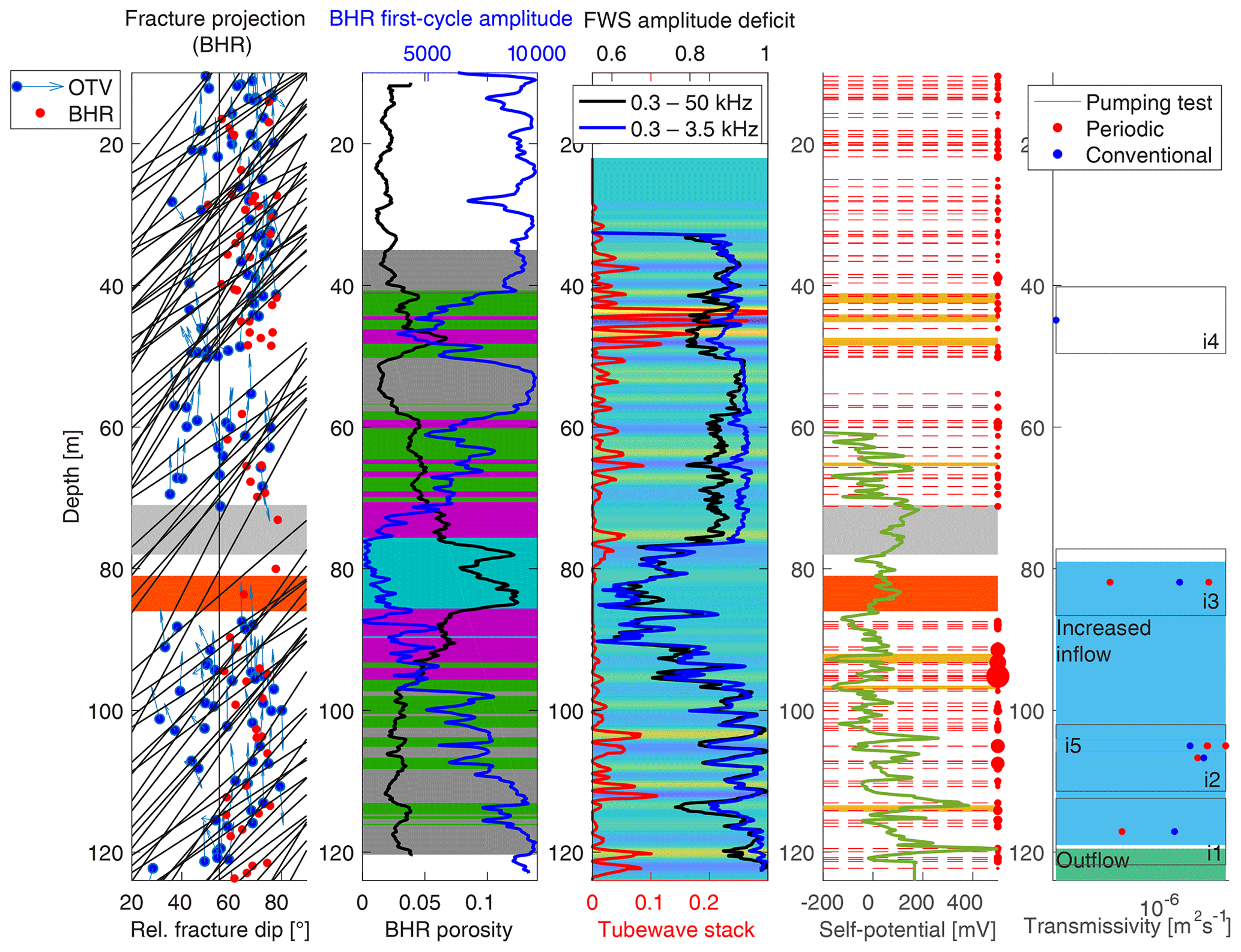
Figure 13From left to right: projection of imaged BHR reflections onto the borehole track together with associated dip, tadpoles illustrating the azimuth, and dip for the fractures identified from the OTV data; results of cluster analysis overlain by BHR porosity and BHR amplitudes; tube wave stack overlain by tube wave energy (Greenwood et al., 2019) and Stoneley energy deficit; brittle deformation data overlain by the corrected SP log (2017); and summary of transmissivities estimated from pumping tests (Cheng and Renner, 2017).
Table 3Petrophysical properties of the cluster groups (25th and 75th percentile) and core measurements.

a Jörg Renner (personal communication, 2016), b Ultrasonic measurements for saturated (and dry) samples under ambient conditions (Jörg Renner, personal communication, 2018), c Egli et al. (2018) multiscale analysis.
Although there are uncertainties in the absolute values of the measurements due to borehole enlargements, the relative variations in the petrophysical properties are clearly dominated by the different degrees of brittle deformation. Table 3 summarizes the range (25th and 75th percentiles of the median) of porosity and P- and S-wave velocities for the groups identified in the cluster analysis and compares them to core measurements and average matrix and micro-fracture porosity estimates of Egli et al. (2018). These authors differentiate matrix porosity types by their mineralogy and texture. Quartz-dominated zones are governed by inter- and intragranular porosity (0.8 %), feldspar-dominated areas by solution porosity (1.4 %), fine-grained mica (75 µm) and coarse grained mica by inter- and intragranular porosity (2.8 % and 4.6 %), whereas breccia porosity is significantly higher. A summary of their estimates for mean matrix and fracture porosity is provided in Table 3. These estimates obviously do not account for larger fractures, which are captured by the log data. Nevertheless, for the cataclasites and the fault breccia the mean porosity estimates fall within the range of values obtained for clusters 1 and 2, which are categorized as the main fault core and regions of high fracture density or cataclastic zones, respectively. The values for clusters 3 and 4, which cover sections of the borehole with moderate to low fracture density, are quite similar to mean matrix and micro-fracture porosity values of the granites, gneisses and mylonites. However, a more detailed differentiation between these tectonic groups based on the log data is not possible. Ultrasonic velocity measurements performed on selected core samples generally provide higher values than the sonic log measurements. However, the maximum velocity values of the sonic log data in cluster 4, which comprises the most intact rocks, fall within the range of these laboratory measurements. The chosen core samples cover different types of fabric variations (granitoids, gneiss, and mylonites) and are from the more intact parts of the recovered drill core. Nevertheless, even these core samples still seem to contain fractures, as evidenced by the non-negligible difference between dry and saturated ultrasonic P-wave velocity measurements. This suggests that the elastic response of the damage zone of the GBF is dominated by the mechanical compliance of fractures at multiple scales.
The energy deficit of the Stoneley wave is related to the hydraulic transmissivity. At lower frequencies, this wave type is referred to as a tube wave and commonly encountered in hydrophone VSP surveys. Greenwood et al. (2019) linked the tube waves along the GDP1 borehole to hydraulically open fractures. Figure 13 compares the tube wave energy along the borehole with the energy deficit of the low-frequency FWS data. Both measures respond to hydraulically open fractures along the borehole. For the cataclastic zones and some of the large-scale fractures, we observe a good correlation between the two energy measures. In the zone around the main fault core, the agreement is less good, since borehole enlargements and the rugosity of the borehole wall prevent the propagation of tube waves. However, tube waves are still created in this region as shown by Greenwood et al. (2019). Thus suggesting that these are zones/features of increased hydraulic transmissivity. Furthermore, the distinct anomalies in the wave energy deficit in the damage zone below the GBF show a very good correlation with the anomalies encountered in the SP data. This supports our interpretation that the SP anomalies are related to fluid flow governed by hydraulically open fractures.
For specifically targeted zones, indicated in Fig. 13, Cheng and Renner (2017) performed conventional and periodic pumping tests in the GDP1 borehole in 2015. The resulting transmissivity estimates are shown in Fig. 13. The highest values are obtained for the intervals i2 and i5, which feature a large aperture fracture of 16.4 mm at 105 m borehole depth. This fracture can be associated with a distinct anomaly in the SP data and the energy deficit. However, no clear trend can be established between the magnitude of the anomalies in the two log attributes and the estimated transmissivity from the pumping tests. One reason is that the pumping test only provides a few values of transmissivity averaged over relatively large intervals. The logs analyzed in this study do, however, point to a compartmentalized system with distinct hydraulic zones with water of different origins. A hypothesis is the existence of a shallow water reservoir above 95 m depth where meteoric water penetrates into the formation through the exposed fracture network, whereas below 95 m depth, a deeper and more saline hydrothermal water reservoir may prevail. Even though, there is no clear evidence of a hydraulic barrier between the two zones, below 95 m depth, a zone of increased ductile deformation with fracture apertures smaller than 3 mm followed by a zone of weakly deformed granite may act as such a barrier. Furthermore, the results of Cheng and Renner (2017) suggest a complex and variable flow geometry on the decameter scale in the studied subsurface region of the GBF associated with a heterogeneous system dominated by steeply dipping structures with a pipe-like hydraulic behavior. No chemical analysis of the water in the GDP1 borehole was conducted. However, the interpretation of different water sources is consistent with a recent hydrogeochemical study (Diamond et al., 2018; Wanner et al., 2019) carried out in the Transitgas AG tunnel situated 200 m below the GDP1 borehole. The study identified two types of springs along the tunnel: (i) cold springs with a low mineralization (total dissolved solids TDS < 100 mg L−1) and (ii) warm springs with elevated mineralization (TDS > 250 mg L−1). The composition of the warm springs can be well explained by a binary mixture between a geothermal component characterized by elevated salinity and temperature and weakly mineralized cold meteoric water from the surface.
All of this points to the presence of distinctively different sources and passages of fluid flow in the studied subsurface region of the GBF (GDP1 borehole), thus suggesting a compartmentalization of fluid pathways in the hydraulic system along steeply dipping intersecting fractures and cataclastic zones. The main flow paths are associated with the intensely fractured nature of the exhumed ductile shear zone. Fracture permeability is expected to decrease with depth due to its inherent pressure-dependence, but cataclastic zones may retain a part of their porosity due to hydrothermal processes. Furthermore, Egli et al. (2018) suggested that fault intersections act as regions of high permeability in the Grimsel Pass hydrothermal zones. These intersections inferred from the drill hole data and observed in the BHR data may prevail on a larger scale along the GBF, effectively feeding a hydrothermal reservoir with meteoric water and allowing localized upflow of hydrothermal water along cataclastic zones (subsidiary fault cores) and fault intersections (Egli et al., 2018). This interpretation is supported by the study of Belgrano et al. (2016), which analyzed the architecture and hydrothermal activity of the GBF on a larger scale and concluded that the hydraulic characteristics are controlled by localized subvertically oriented pipe-like upflow zones. Furthermore, a recent study of Wanner et al. (2019) based on 3D thermal-hydraulic modeling constrained by surface observations of warm springs and fossil hydrothermal mineralization, suggested that the thermal anomaly at the Grimsel Pass may reach down to 9 km depth. The authors did, however, argue that, this specific anomaly is not a suitable candidate for petrothermal power production due to its comparatively low flow rates.
With the objective to characterize the fracture network of the damage zone surrounding the GBF and its petrophysical properties, we have performed an integrated analysis of the geophysical borehole log measurements. Although the log data are affected by challenging borehole conditions, notably numerous and large enlargements, the dataset contains a multitude of valuable information, which is in agreement with previous studies and adds to their findings. The BHR reflection data in combination with the OTV data suggest a complex network of fluid-filled fractures in the damage zone surrounding the main fault core of the GBF. Larger-scale fractures can be tracked several meters into the formation in the BHR reflection image, which, in turn, confirms that the borehole enlargements can generally be related to geological features and are not primarily drilling-induced damage. A comparison of the borehole logs to the fracture characteristics inferred from the OTV data confirms that the response of the logs, and thus the variations in petrophysical properties, are predominantly governed by the intensity of brittle deformation. A clear influence of ductile deformation on the petrophysical properties cannot be discerned. Overall, the measured petrophysical properties correlate very well with each other. Many of the petrophysical properties show distinctly different values than those expected for intact granitic formations, such as P-wave and S-wave velocities ranging between 2600 to 5600 and 1600 to 3200 m s−1, respectively, and porosities ranging between 3 % and 15 %. The compliant high-porosity zones associated with cataclastic structures and fractures are the main fluid pathways of the system. The SP data show an abundance of anomalies, which can be linked to fractures and are most likely of electrokinetic origin. The results of the SP probability tomography suggest that above 95 m inflow is dominating, and below inflow and outflow occurs with a dominant outflow region around 120 m borehole depth. Furthermore, the distinct layering observed in the fluid resistivity points to a compartmentalized pipe-like hydraulic behavior dominated by the steeply dipping geological structures as well as to the inflow of water from various different sources.
To derive reliable porosity estimates from the first-arrival travel times of the BHR data, we have to apply a zero-time correction. For the data collected in 2015, a zero-time correction was not available. Thus, we used the corresponding information for the 2016 data (Fig. A1) to first correct the 2016 picks (Fig. A2). This is followed by a static shift of the 2015 picks corresponding to the mean difference in travel times with regard to the corrected 2016 picks. The resulting corrected travel times of the 2015 BHR data are shown in Fig. A2 and are used for the porosity estimation in Sect. 5.1.
To downscale the porosity estimates obtained from the BHR data, we utilize the neutron–neutron log. Therefore, we calibrate the neutron–neutron log with the BHR porosity estimates above and below the main fault core by fitting a power-law relationship. The calibration interval is shown in Fig. A3a and the resulting fit in Fig. A3b. The data in Fig. A3b is displayed in terms of a histogram crossplot. For comparison, we have also plotted porosities measured in the laboratory for selected core samples, which are in good agreement with the data fit. Subsequently, we used the inferred power law to convert the counts of the neutron–neutron log into porosities along the entire borehole.
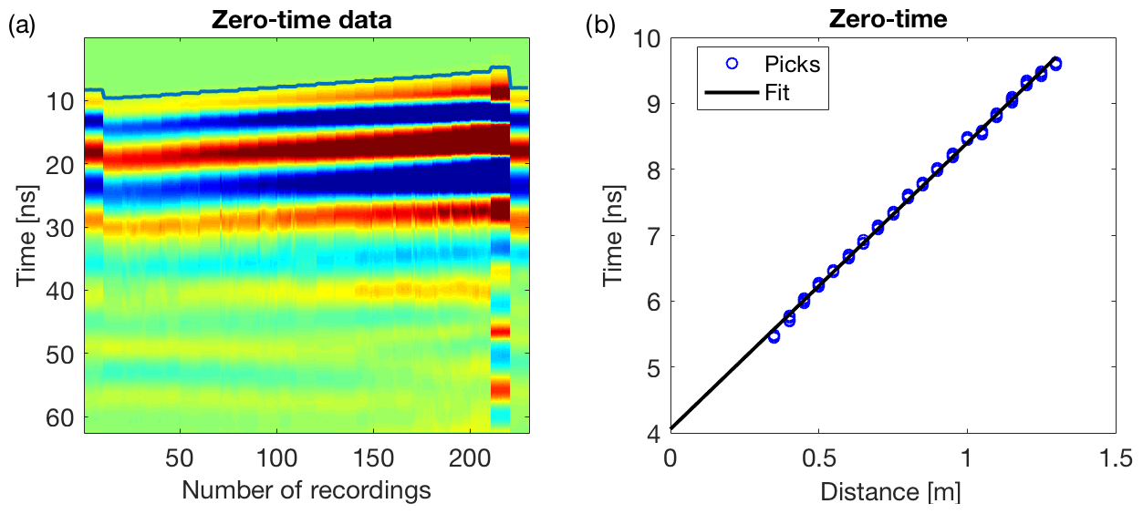
Figure A1(a) Data collected in 2016 for zero-time correction showing 10 recordings per distance as well as the first arrival picks. (b) Picked first arrivals vs. distance with the corresponding linear regression fit. First and last 10 stacks are not considered.
As mentioned in Sect. 5 Archie's law is not suitable to estimate porosity from the resistivity data. To illustrate this we plot in Fig. A4 the formation factor calculated from the normal resistivity measurements of 16 in. (0.4 m) and 32 in. (0.8 m) (recorded in 2016) and the fluid resistivity obtained from the STS measurement at ambient conditions (2016) as a function of the porosity estimates obtained from the BHR data. For the comparison depth intervals above and below the main fault zone are chosen. The data clearly plots outside the validity range of Archie's law (Fig. A4) and exhibits a different functional relationship between the formation factor and porosity than the simple power law of Archie. One possible reason might be the influence of surface conductivity. Interestingly the data in the upper section of the borehole (42–72 m) would suggest a higher matrix conductivity than in the lower part of the borehole (105–120 m). The upper section contains stronger ductile deformation and thus more mylonitic zones. A recent study of electrical properties of mylonites from the Alpine Fault project in New Zealand found values ranging from 675 to 75 Ω m (Kluge et al., 2017).

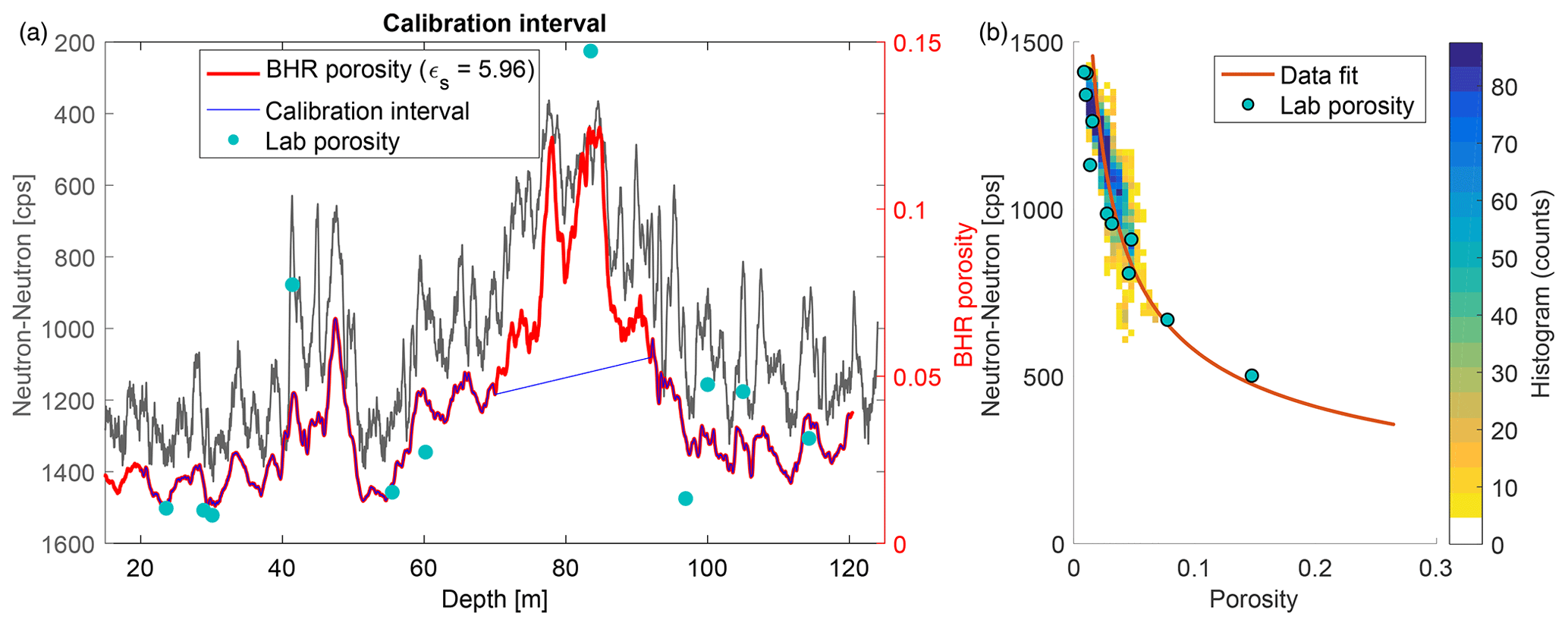
Figure A3(a) Neutron–neutron counts and best-fitting BHR porosity. (b) Fitted relation between the neutron–neutron and the BHR porosity overlaying a corresponding histogram crossplot.

Figure A4Formation factor vs. porosity obtained from the borehole radar for a permittivity of the solid of 5.69. The formation factor is calculated from the normal resistivity measurements of 16 in. (0.4 m) and 32 in. (0.8 m) (2016) and the fluid resistivity obtained from the STS measurement at ambient conditions (2016). For comparison Archie's law with a cementation factor of m=1 and m=2 is shown.
The resistivity logs were acquired in 3 consecutive years. The 2015 data correspond to open-hole conditions. They are affected by the pumping of lake water into the borehole as well as by the remnants of polymer-based drilling mud in the formation. Conversely, the 2016 and 2017 data were measured through slotted PVC casing. As a result, the logs contain spikes at the positions of the casing joints as illustrated in Fig. B1 for the normal resistivity, single point resistance, and SP data. We corrected the data by removing the spikes and subsequent linear interpolation of the gaps. For the normal resistivity data, we recovered the variability in the logs by replacing the interpolated sections with the 2015 data shifted to the respective baseline of the 2016 or 2017 data (Toschini, 2018). The resulting logs are shown in Fig. B2.
The SP measurements are additionally affected by a very strong drift, since the steel cable suspending the tool serves as the reference electrode. The data are unusable until the exposed cable is ∼30 m below the water level. Since the water table was at ∼33 m borehole depth at the time of the measurements in 2016 and 2017, the logs can only be used from ∼60 m onwards. To compensate for the remaining drift in the data below ∼60 m borehole depth, we remove a linear background trend for each dataset separately instead of normalizing the data to a constant baseline value (Fig. B1).
Figure B2 shows a selection of the casing-corrected resistivity data measured in 2016 and 2017 in comparison to the 2015 open-hole data. Across all 3 years, the normal resistivity (N16) measurements are consistent. The biggest differences occur in the high-porosity zone A and around the cementation region of the borehole. The most likely reason is a change in water resistivity possibly due to the drilling mud. Toschini (2018) performed a modeling study to account for the effect of the PVC casing on the resistivity values after correcting for the joints and found that the impact was not significant.
The single-point resistivity measurements allow the detection of individual fractures more precisely than normal resistivity measurements, but they are very sensitive to the fluid resistivity, which was significantly different in 2015 compared to the other 2 years. There are differences between the 2015 and the 2016/2017 logs around 70 to 86 and 113 to 122 m borehole depth, which most likely are due to the remnant presence of drilling fluid in the adjacent formation as well as to the pumping of lake water into the borehole. Interestingly, a series of repeat measurements in 2015 showed that, in these two zones, the fluid resistivity equilibrates more slowly than in other zones of the borehole. Furthermore, the single-point resistivity logs seem to be more strongly affected by the PVC casing and are generally noisier than the normal resistivity measurements.
For the SP data, we observe a marked difference between the data acquired in 2015 and those acquired in 2016 and 2017. The 2015 dataset is quite noisy, and the only anomaly visible is in the vicinity of the cemented zone. One reason for the difference between the datasets might again be the remnant presence of polymer-based drilling mud, which changed the viscosity and the chemical composition of the water in the adjacent formation. Apart from this, lake water was pumped into the borehole. This raised the water level to ∼8 m borehole depth, which is 20 m above the ambient levels found in 2016 and 2017. Correspondingly, the SP data measured in 2015 do not reflect hydraulic steady-state conditions of the borehole and its vicinity.

Figure B1Comparison of open- and cased-hole data. From left to right: normal resistivity, single-point resistance, and SP logs for 2015, 2016, and 2017 with casing joints marked in grey, casing-corrected SP log, and background-trend-corrected SP log.

The data can be downloaded at https://github.com/rockphysicsUNIL/GDP1_Well_log_data (Caspari, 2020) and are also available upon request.
EC was responsible for data processing, analysis, and interpretation and preparation of the paper. AG was responsible for data acquisition and conditioning, processing of borehole radar data, and contributing to the overall data interpretation. LB was responsible for the design of the logging campaign, data acquisition, and support with the data analysis. DE was responsible for geological interpretation, analysis of the OTV data, and porosity estimation from image analysis. ET was responsible for acquisition and processing of the normal resistivity data. KH was responsible for probability tomography of the self potential data and support with the interpretation of the self potential data. KH was responsible for project leadership, contributions to data interpretation, and paper preparation.
The authors declare that they have no conflict of interest.
This work was supported by the Swiss National Science Foundation through the National Research Programme 70 “Energy Turnaround” and completed within the Swiss Competence Center on Energy Research – Supply of Electricity, with the support of the Swiss Innovation Agency. We thank Tobias Zahner for his active involvement in the 2015 and 2016 data acquisition campaign, Yannick Forth and Jörg Renner from Ruhr-University Bochum for providing Archimedes type density measurements and porosity measurements performed on the core samples, and Jörg Renner for the ultrasonic velocity measurements.
This research has been supported by the Swiss National Science Foundation (grant no. 407040_153889).
This paper was edited by Charlotte Krawczyk and reviewed by Thomas Doe and one anonymous referee.
Ahlbom, K., Smeallie, J., Tirén, S., Andersson, J.-E., Ekman, L., Nordquist, R., Wikberg, P., Andersson, P., and Gustafsson, E.: Characterization of fracture zone 2, Finnsjön study-site, SKB Technical Report 89-19, Tech. rep., Svensk Kärnbränslehantering AB, Swedish Nuclear Fuel and Waste Management Co., 1989. a
Arthur, D. and Vassilvitskii, S.: k-means++: The advantages of careful seeding, in: Proceedings of the eighteenth annual ACM-SIAM symposium on Discrete algorithms, 1027–1035, Society for Industrial and Applied Mathematics, 2007. a
Barbosa, N. D., Caspari, E., Rubino, J. G., Greenwood, A., Baron, L., and Holliger, K.: Estimation of fracture compliance from attenuation and velocity analysis of full-waveform sonic log data, J. Geophys. Res.-Sol. Ea., 124, 2738–2761, 2019. a
Barton, C. A., Zoback, M. D., and Moos, D.: Fluid flow along potentially active faults in crystalline rock, Geology, 23, 683–686, 1995. a, b
Belgrano, T. M., Herwegh, M., and Berger, A.: Inherited structural controls on fault geometry, architecture and hydrothermal activity: an example from Grimsel Pass, Switzerland, Swiss J. Geosci., 109, 345–364, 2016. a, b, c, d, e, f
Berkowitz, B.: Characterizing flow and transport in fractured geological media: A review, Adv. Water Resour., 25, 861–884, 2002. a, b
Brace, W.: Permeability of crystalline and argillaceous rocks, in: International Journal of Rock Mechanics and Mining Sciences & Geomechanics Abstracts, Vol. 17, 241–251, Elsevier, Pergamon, 1980. a
Bradford, J. H., Clement, W. P., and Barrash, W.: Estimating porosity with ground-penetrating radar reflection tomography: A controlled 3-D experiment at the Boise Hydrogeophysical Research Site, Water Resour. Res., 45, 2009. a
Caine, J. S., Evans, J. P., and Forster, C. B.: Fault zone architecture and permeability structure, Geology, 24, 1025–1028, 1996. a
Caspari, E.: GDP1 well log data from a hydrothermally altered shear zone, available at: https://github.com/rockphysicsUNIL/GDP1_Well_log_data, last access: 17 March 2020. a
Cheng, Y. and Renner, J.: Exploratory use of periodic pumping tests for hydraulic characterization of faults, Geophys. J. Int., 212, 543–565, 2017. a, b, c, d, e, f, g, h
Diamond, L. W., Wanner, C., and Waber, H. N.: Penetration depth of meteoric water in orogenic geothermal systems, Geology, 46, 1063–1066, 2018. a, b
Di Maio, R. and Patella, D.: Self-potential anomaly generation in volcanic areas. The Mt, Etna case-history, Acta Vulcanol., 4, 119–124, 1994. a
Dorn, C., Linde, N., Doetsch, J., Le Borgne, T., and Bour, O.: Fracture imaging within a granitic rock aquifer using multiple-offset single-hole and cross-hole GPR reflection data, J. Appl. Geophys., 78, 123–132, 2012. a
Egli, D., Baumann, R., Küng, S., Berger, A., Baron, L., and Herwegh, M.: Structural characteristics, bulk porosity and evolution of an exhumed long-lived hydrothermal system, Tectonophysics, 747, 239–258, 2018. a, b, c, d, e, f, g, h, i, j, k, l, m, n, o, p, q, r, s, t, u, v, w
Ellis, D. V. and Singer, J. M.: Well logging for earth scientists, Vol. 692, Springer, Dordrecht, 2007. a
Evans, J. P., Forster, C. B., and Goddard, J. V.: Permeability of fault-related rocks, and implications for hydraulic structure of fault zones, J. Struct. Geol., 19, 1393–1404, 1997. a
Evans, K. F., Genter, A., and Sausse, J.: Permeability creation and damage due to massive fluid injections into granite at 3.5 km at Soultz: 1. Borehole observations, J. Geophys. Res.-Sol. Ea., 110, B04203, https://doi.org/10.1029/2004JB003168, 2005. a
Faulkner, D. and Armitage, P.: The effect of tectonic environment on permeability development around faults and in the brittle crust, Earth Planet. Sc. Lett., 375, 71–77, 2013. a
Genter, A., Castaing, C., Dezayes, C., Tenzer, H., Traineau, H., and Villemin, T.: Comparative analysis of direct (core) and indirect (borehole imaging tools) collection of fracture data in the Hot Dry Rock Soultz reservoir (France), J. Geophys. Res.-Sol. Ea., 102, 15419–15431, 1997. a
Glover, P.: Geophysical properties of the near surface Earth: Electrical properties, in: Treatise on Geophysics, 2nd Edn., 89–137, Elsevier, Oxford, 2015. a
Greaves, R. J., Lesmes, D. P., Lee, J. M., and Toksöz, M. N.: Velocity variations and water content estimated from multi-offset, ground-penetrating radar, Geophysics, 61, 683–695, 1996. a
Greenwood, A., Caspari, E., Egli, D., Baron, L., Zahner, T., Hunziker, J., and Holliger, K.: Characterization and imaging of a hydrothermally active near-vertical fault zone in crystalline rocks based on hydrophone VSP data, Tectonophysics, 750, 153–176, 2019. a, b, c, d, e
Hämmann, M., Maurer, H., Green, A., and Horstmeyer, H.: Self-potential image reconstruction: capabilities and limitations, J. Environ. Eng. Geoph., 2, 21–35, 1997. a
Himmelsbach, T., Shao, H., Wieczorek, K., Flach, D., Schuster, K., Alheid, H.-J., Liou, T.-S., Bartlakowski, J., and Krekeler, T.: Grimsel Test Site Investigation Phase V Effective Field Parameter EFP, Technischer Bericht-NAGRA NTB, 2003. a
Hobday, C. and Worthington, M.: Field measurements of normal and shear fracture compliance, Geophys. Prospect., 60, 488–499, 2012. a
Hofmann, B. A., Helfer, M., Diamond, L. W., Villa, I. M., Frei, R., and Eikenberg, J.: Topography-driven hydrothermal breccia mineralization of Pliocene age at Grimsel Pass, Aar massif, Central Swiss Alps, Schweiz. Miner. Petrog., 84, 271–302, 2004. a, b, c, d
Holbrook, W. S., Mooney, W. D., and Christensen, N. I.: The seismic velocity structure of the deep continental crust, in: Continental Lower Crust, Developments in Geotectonics, edited by: Fountain, D. M., Arculus, R., and Kay, R. W., 1–43, Elsevier, Amsterdam, 1992. a
Hornby, B. E.: Imaging of near-borehole structure using full-waveform sonic data, Geophysics, 54, 747–757, 1989. a
Iuliano, T., Mauriello, P., and Patella, D.: Looking inside Mount Vesuvius by potential fields integrated probability tomographies, J. Volcanol. Geoth. Res., 113, 363–378, 2002. a
Jackson, M.: Tools and techniques: Self-potential methods, in: Treatise on Geophysics, 2nd Edn., 261–293, Elsevier, Oxford, 2015. a, b
Keys, W. S. and Sullivan, J. K.: Role of borehole geophysics in defining the physical characteristics of the Raft River geothermal reservoir, Idaho, Geophysics, 44, 1116–1141, 1979. a
Kluge, K., Toy, V., Ohneiser, C., and Lockner, D.: Electrical properties of schist and mylonite from the South Island, New Zealand: Exploring the source of the Southern Alps Anomalous Conductor, Geophys. Res. Abstr., EGU2017-10139, EGU General Assembly 2017, Vienna, Austria, 2017. a, b
Liu, E. and Martinez, A.: Seismic fracture characterization, EAGE, Oxford, 2014. a
Loew, S., Barla, G., and Diederichs, M.: Engineering geology of Alpine tunnels: Past, present and future, in: Geologically active, Proceedings of the 11th IAEG Congress, 201–253, CRC press, Auckland, NZ, 2010. a
Mauriello, P. and Patella, D.: Resistivity anomaly imaging by probability tomography, Geophys. Prospect., 47, 411–429, 1999. a
Nelson, R. A.: Geological analysis of naturally fractured reservoirs, 2nd Edn., Gulf Professional Publishing, Woburn, 2001. a
Olsson, O., Falk, L., Forslund, O., Lundmark, L., and Sandberg, E.: Borehole radar applied to the characterization of hydraulically conductive fracture zones in crystalline rock 1, Geophys. Prospect., 40, 109–142, 1992. a
Paillet, F. L.: Acoustic characterization of fracture permeability at Chalk River, Ontario, Can. Geotech. J., 20, 468–476, 1983. a
Paillet, F. L.: Application of borehole geophysics in the characterization of flow in fractured rocks, Water-Resources Investigations Report, 93, 4214, https://doi.org/10.3133/wri934214, 1994. a, b
Prioul, R. and Jocker, J.: Fracture characterization at multiple scales using borehole images, sonic logs, and walkaround vertical seismic profile, AAPG Bull., 93, 1503–1516, 2009. a
Regenauer-Lieb, K., Bunger, A., Chua, H. T., Dyskin, A., Fusseis, F., Gaede, O., Jeffrey, R., Karrech, A., Kohl, T., Liu, J., Lyakhovsky, V., Pasternak, E., Podgorney, R., Poulet, T., Rahman, S., Schrank, C., Trefry, M., Veveakis, M., Wu, B., Yuen, D. A., Wellmann, F., and Zhang, X.: Deep geothermal: The “Moon Landing” mission in the unconventional energy and minerals space, J. Earth Sci., 26, 2–10, 2015. a
Revil, A., Naudet, V., Nouzaret, J., and Pessel, M.: Principles of electrography applied to self-potential electrokinetic sources and hydrogeological applications, Water Resour. Res., 39, 1114, https://doi.org/10.1029/2001WR000916, 2003. a
Salisbury, M. H., Harvey, C. W., Matthews, L., Eaton, D., and Milkereit, B.: The acoustic properties of ores and host rocks in hardrock terranes, Hardrock seismic exploration, edited by: Eaton, D. W., Milkereit, B., and Salisbury, M. H., Society of Exploration Geophysicists, Tulsa, Okla, 9–19, 2003. a
Saracco, G., Labazuy, P., and Moreau, F.: Localization of self-potential sources in volcano-electric effect with complex continuous wavelet transform and electrical tomography methods for an active volcano, Geophys. Res. Lett., 31, L12610, https://doi.org/10.1029/2004GL019554, 2004. a
Schmitt, D. R., Mwenifumbo, C. J., Pflug, K. A., and Meglis, I. L.: Geophysical logging for elastic properties in hard rock: a tutorial, Hardrock seismic exploration, edited by: Eaton, D. W., Milkereit, B., and Salisbury, M. H., Society of Exploration Geophysicists, Tulsa, Okla, 20–42, 2003. a
Sonney, R. and Vuataz, F.-D.: Properties of geothermal fluids in Switzerland: a new interactive database, Geothermics, 37, 496–509, 2008. a
Stephens, M. B., Follin, S., Petersson, J., Isaksson, H., Juhlin, C., and Simeonov, A.: Review of the deterministic modelling of deformation zones and fracture domains at the site proposed for a spent nuclear fuel repository, Sweden, and consequences of structural anisotropy, Tectonophysics, 653, 68–94, 2015. a
Suski, B., Ladner, F., Baron, L., Vuataz, F.-D., Philippossian, F., and Holliger, K.: Detection and characterization of hydraulically active fractures in a carbonate aquifer: results from self-potential, temperature and fluid electrical conductivity logging in the Combioula hydrothermal system in the southwestern Swiss alps, Hydrogeol. J., 16, 1319–1328, 2008. a
Tibshirani, R., Walther, G., and Hastie, T.: Estimating the number of clusters in a data set via the gap statistic, J. R. Stat. Soc. B, 63, 411–423, 2001. a
Toschini, E.: Exploration et caractérisation d'une zone hydrothermale fracturée active: acquisition, traitement et interprétation de mesures géoelectriques dans un puits, Master's thesis, University of Lausanne, 2018. a, b, c
Townend, J., Sutherland, R., Toy, V., Eccles, J., Boulton, C., Cox, S., and McNamara, D.: Late-interseismic state of a continental plate-bounding fault: Petrophysical results from DFDP-1 wireline logging and core analysis, Alpine Fault, New Zealand, Geochem. Geophy. Geosy., 14, 3801–3820, 2013. a
Valley, B. C.: The relation between natural fracturing and stress heterogeneities in deep-seated crystalline rocks at Soultz-sous-Forêts (France), PhD thesis, ETH Zurich, 2007. a, b
Wanner, C., Diamond, L. W., and Alt-Epping, P.: Quantification of 3-D Thermal Anomalies From Surface Observations of an Orogenic Geothermal System (Grimsel Pass, Swiss Alps), J. Geophys. Res.-Sol. Ea., 124, 10839–10854, 2019. a, b, c
- Abstract
- Introduction
- Geological setting and borehole conditions
- Borehole radar reflection data: imaging of the fracture network
- Characteristics of the damage zone from geophysical logs
- Porosity distribution and fluid flow characteristics
- Discussion
- Conclusions
- Appendix A
- Appendix B
- Data availability
- Author contributions
- Competing interests
- Acknowledgements
- Financial support
- Review statement
- References