the Creative Commons Attribution 4.0 License.
the Creative Commons Attribution 4.0 License.
 | 05 Feb 2019
Power spectra of random heterogeneities in the solid earth
Haruo Sato
Recent seismological observations focusing on the collapse of an impulsive wavelet revealed the existence of small-scale random heterogeneities in the earth medium. The radiative transfer theory (RTT) is often used for the study of the propagation and scattering of wavelet intensities, the mean square amplitude envelopes through random media. For the statistical characterization of the power spectral density function (PSDF) of the random fractional fluctuation of velocity inhomogeneities in a 3-D space, we use an isotropic von Kármán-type function characterized by three parameters: the root mean square (RMS) fractional velocity fluctuation, the characteristic length, and the order of the modified Bessel function of the second kind, which leads to the power-law decay of the PSDF at wavenumbers higher than the corner. We compile reported statistical parameters of the lithosphere and the mantle based on various types of measurements for a wide range of wavenumbers: photo-scan data of rock samples; acoustic well-log data; and envelope analyses of cross-hole experiment seismograms, regional seismograms, and teleseismic waves based on the RTT. Reported exponents of wavenumber are distributed between −3 and −4, where many of them are close to −3. Reported RMS fractional fluctuations are on the order of 0.01–0.1 in the crust and the upper mantle. Reported characteristic lengths distribute very widely; however, each one seems to be restricted by the dimension of the measurement system or the sample length. In order to grasp the spectral characteristics, eliminating strong heterogeneity data and the lower mantle data, we have plotted all the reported PSDFs of the crust and the upper mantle against wavenumber for a wide range (10−3–108 km−1). We find that the spectral envelope of those PSDFs is well approximated by the inverse cube of wavenumber. It suggests that the earth-medium randomness has a broad spectrum. In theory, we need to re-examine the applicable range of the Born approximation in the RTT when the wavenumber of a wavelet is much higher than the corner. In observation, we will have to carefully measure the PSDF on both sides of the corner. We may consider the obtained power-law decay spectral envelope as a reference for studying the regional differences. It is interesting to study what kinds of geophysical processes created the observed power-law spectral envelope at different scales and in different geological environments in the solid earth medium.
- Article
(3345 KB) - Full-text XML
- BibTeX
- EndNote


The first image of the solid earth is composed of spherical shells, for example, PREM (preliminary reference Earth model) (Dziewonski and Anderson, 1981). As seismic networks were deployed on the regional scale and worldwide, the velocity tomography based on the ray tracing method revealed 3-D heterogeneous structures at various scales; however, spatial variations in the resultant velocity structure are essentially smooth compared with seismic wavelengths. Aki and Chouet (1975) first put a focus on long-lasting coda waves of small earthquakes and interpreted them as scattered waves by small-scale random heterogeneities. They proposed to measure the scattering coefficient g, the scattering power per unit volume as a measure of medium heterogeneity. They analyzed the mean square (MS) amplitude time trace of coda waves as an incoherent sum of scattered wave power by using the Born approximation (e.g., Chernov, 1960), which is a simplified version of the radiative transfer theory (RTT). There have been many measurements of the total scattering coefficient giso supposing isotropic scattering (e.g., Sato, 1977a) in various seismotectonic environments. The total scattering coefficient of S waves is reported to be on the order of 10−2 km−1 for 1–20 Hz in the lithosphere, and it marks a higher value beneath active volcanoes (e.g., Sato et al., 2012; Yoshimoto and Jin, 2008). There were precise measurements of regional variations in giso as Carcolé and Sato (2010) in Japan and Eulenfeld and Wegler (2017) in the US. Hock et al. (2004) analyzed medium heterogeneity in Europe from the analyses of teleseismic waves using the modified energy flux model (Korn, 1993). There were also measurements of the anisotropic scattering coefficient from the analysis of S coda envelopes Jing et al. (e.g., 2014); Zeng (e.g., 2017).
Aki and Chouet (1975) derived the angular dependence of the scattering coefficient of scalar waves from the power spectral density function (PSDF) of the fractional velocity fluctuation using the Born approximation. Sato (1984) extended the envelope synthesis of scalar waves to the whole envelope synthesis of three-component seismograms from the P onset to S coda on the bases of the single scattering approximation of the RTT. His syntheses explain how seismogram envelopes in different back azimuths vary depending on the source fault mechanism. Extension to the multiple scattering case was developed by using Stokes parameters (e.g., Margerin et al., 2000; Margerin, 2005; Przybilla et al., 2009; Sanborn et al., 2017). We also note that Monte Carlo simulation was developed to stochastically solve the RTT (e.g., Hoshiba et al., 1991; Gusev and Abubakirov, 1987; Yoshimoto, 2000). For the data processing, it is more appropriate to stack MS envelopes of observed seismograms for comparison with the averaged intensity time traces stochastically synthesized by the RTT (e.g., Shearer and Earle, 2004; Rost et al., 2006; da Silva et al., 2018).
When the central wavenumber of a wavelet increases much larger than the corner wavenumber of the PSDF, the wavelet around the peak value is mostly composed of narrow-angle scattering around the forward direction. In such a case, the Born approximation becomes inappropriate; however, the phase shift modulation based on the parabolic approximation is useful, which is called the phase screen approximation. As an extension of the RTT with the phase screen approximation, the Markov approximation was also used for the analysis of envelope broadening and peak delay with increasing travel distance (e.g., Sato, 1989; Saito et al., 2002; Takahashi et al., 2009). Kubanza et al. (2007) measured regional differences in the lithospheric heterogeneity from the partitioning of seismic energy of teleseismic P waves into the vertical and transverse components based on the Markov approximation.
There have been various kinds of measurements of the PSDF of the random velocity fluctuation, where the PSDF is often supposed to be a von Kármán type. In the following section, the main objective is to compile reported PSDF measurements in various scales in different geological environments of the solid earth: photo scanning of small rock samples, acoustic well logs, array analyses of teleseismic waves, waveform analyses using finite difference (FD) simulations, and analyses of seismogram envelopes on the basis of the RTT. We enumerate their statistical parameters and plot their PSDFs against wavenumber. We will show that the envelope of all the PSDFs is well approximated by a power-law decay curve. Then, we will discuss the results obtained and a few problems in the envelope synthesis theory for such random media and the geophysical origin of such power spectra.
We consider the propagation of scalar waves as a simple model, where the inhomogeneous velocity is given by . The fractional fluctuation ξ(x) is supposed to be a random function of space. We imagine an ensemble of random media {ξ(x)}, where 〈ξ(x)〉=0. Angular brackets mean the ensemble average. We suppose that random media are homogeneous and isotropic, then we statistically characterize them by using the autocorrelation function (ACF):
where . The MS fractional fluctuation as a measure of the strength of randomness is supposed to be small, and . The Fourier transform of ACF gives the PSDF:
where wavenumber . In some literature, (2π)−3 is used as a prefactor in the right-hand side of Eq. (2b).
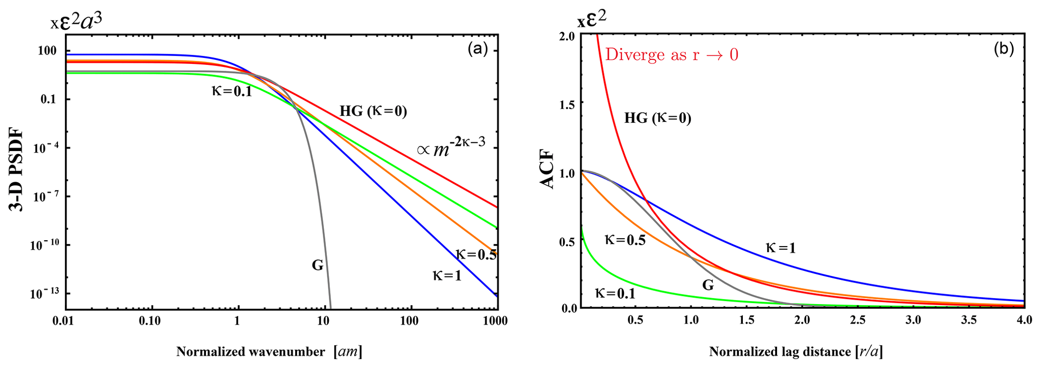
Figure 1(a) Log–log plot of PSDF vs. wavenumber m in 3-D space (von Kármán type, κ=0.1, 0.5, and 1; Henyey–Greenstein type, HG, κ=0; Gaussian type, G). (b) Linear plot of ACF vs. lag distance r.
2.1 Several types of random media
There are several types of PSDF and ACF characterized by a few parameters.
2.1.1 von Kármán type
The ACF is written by using a modified Bessel function of the second kind of order κ and characteristic length a:
which is an exponential type when . In the case of space dimension d, the PSDF is
The PSDF obeys a power-law decay at large wavenumbers: for the 3-D case and for the 1-D case, where κ corresponds to the Hurst number. In the following, we will basically use a von Kármán-type function for characterizing the earth-medium heterogeneity.
Especially for an anisotropic case, we define the von Kármán-type PSDF in 3-D (e.g., Wu et al., 1994; Nakata and Beroza, 2015):
2.1.2 Henyey–Greenstein type
For a case formally corresponding to κ=0 of the von Kármán-type PSDF, we define the Henyey–Greenstein type ACF and PSDF in 3-D (Henyey and Greenstein, 1941):
Note that parameter ε2 characterizes P but ε2≠R(0) since R(r) diverges as r→0.
2.1.3 Gaussian type
Gaussian-type ACF and PSDF are also used because they are mathematically tractable.
We plot those PSDFs against wavenumber and ACFs against lag distance in Fig. 1.
There are several kinds of measurements for estimating statistical parameters characterizing random media. Here we principally collect measurements supposing a von Kármán-type function for isotropic randomness; however, we include a few measurements supposing anisotropic randomness and a Gaussian-type function. On a small scale, the photo-scan method is applied to small rock samples. Acoustic well logs are available in deep wells drilled in the shallow crust. When the precise velocity tomography result is available, we can directly calculate the PSDF. In seismology, the most conventional method is to analyze seismograms of natural earthquakes or artificial explosions after traveling through the earth heterogeneity. It is better to focus on MS amplitude envelopes (intensity time traces) since phases are complex and caused by random heterogeneities. Comparing observed seismogram envelopes with envelopes synthesized in random media, we can evaluate von Kármán parameters. For the synthesis, we can use the FD simulations, the RTT with the Born approximation, and the RTT with the phase screen approximation that is equivalent to the Markov approximation. For each reported measurement, we enumerate the target region, data and the method, the measured PSDF as a function of wavenumber m, von Kármán parameters (κ, ε, a), the frequency range, the wavenumber range, and the reference in Tables 1–3. Note that measurements of heterogeneity listed in the Tables are by no means the only ones. Especially in seismological measurements, we estimate the wave number range from the frequency range by using the typical velocity of the target medium. In the Tables, the parameter values in parentheses (…) are a priori fixed in the measurement. Then, we plot obtained PSDFs against wavenumber in Figs. 2–5. When the estimated parameter value is given by a range, a value in square brackets […] is used to represent for plotting PSDFs in the figures. Measurement with a label with an asterisk * is insufficient for plotting the PSDF in the figures.
Sivaji et al. (2002)Sivaji et al. (2002)Sivaji et al. (2002)Fukushima et al. (2003)Fukushima et al. (2003)Shiomi et al. (1997)Shiomi et al. (1997)Wu et al. (1994)Holliger (1996)Holliger (1996)Table 1Reported von Kaŕmán parameters of rock samples and acoustic well logs. A value in parentheses ( ) is a priori assumed in the measurement. A label with an asterisk * is insufficient for plotting the PSDF.
3.1 Photo scan of the rock surface
The photo-scan method uses a scanner to take a picture of the polished flat surface of a small rock sample (e.g., Sivaji et al., 2002; Spetzler et al., 2002; Fukushima et al., 2003). For the case of a granite sample, those papers classified color images on a straight line into three types of mineral grains: quartz, plagioclase, and biotite. Assigning a typical velocity VP or VS to each mineral grain, they constructed a velocity profile along the line. Then, they estimated the 1-D PSDF of the velocity fractional fluctuation. They measured 1-D PSDFs of granite and gabbro samples fixing κ=0.5 as R1–R5. Figure 2a shows estimated 1-D PSDFs, where the wavenumber range is on the order of 1 mm−1. We note that raw 1-D PSDFs in Figs. 4 and 5 of Fukushima et al. (2003) decay a little slower than those of R4 and R5 in Fig. 2a, especially at large wavenumbers.
3.1.1 Conversion from 1-D PSDF into 3-D PSDF
In the case of isotropic randomness, we evaluate the 1-D PSDF from the 3-D ACF along the z axis at as follows:
Substituting Eq. (3a) into the above equation, we have
Thus, we can evaluate the 3-D PSDF from the 1-D PSDF using parameters ε, κ, and a of 1-D PSDF.
Supposing the randomness is isotropic, we evaluate corresponding 3-D PSDFs of R1–R5 and plot them in Fig. 2b.
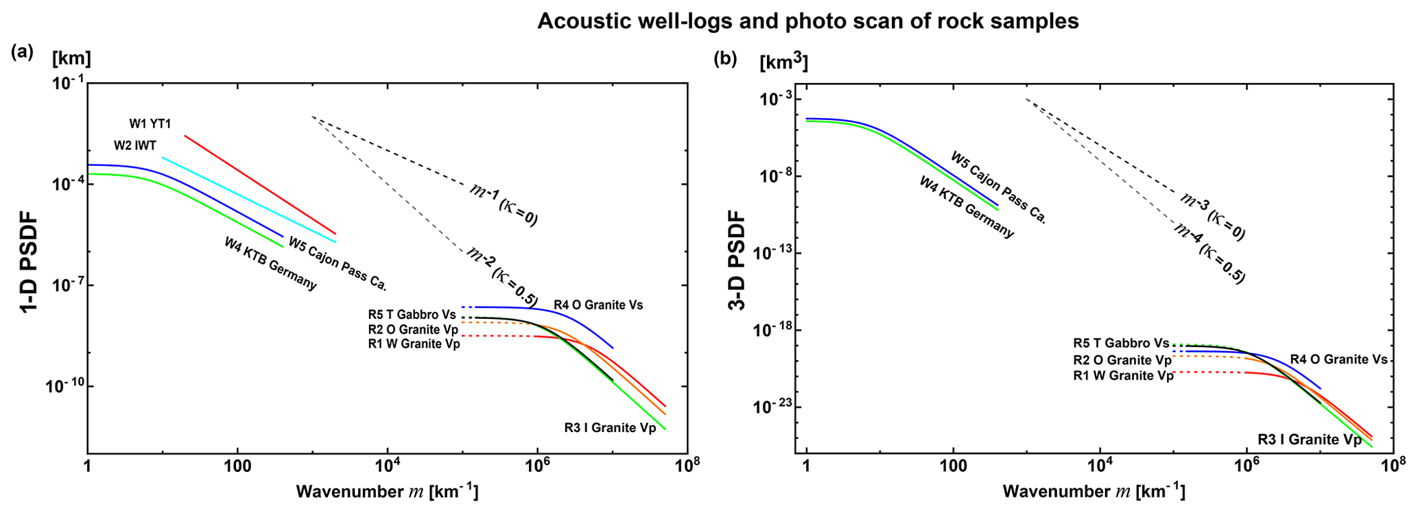
3.2 Acoustic well logs in boreholes
An acoustic well log is obtained from the measurement of the travel time of an ultrasonic pulse along the wall of a borehole. Measurements W1 (volcanic tuff) and W2 (tertiary to pre-tertiary) in Japan clearly show power-law decay with κ=0.225 and 0.045, respectively; however, a corner is not clearly seen in each PSDF. Measurement W4 at the deep well KTB in Germany shows κ=0.10. Measurement W3 in the same well shows that the exponent of wavenumber is −0.97, which formally corresponds to a negative κ. Measurement W5 at Cajon Pass in California shows κ=0.11. All these measurements show very small κ values close to 0. Shiomi et al. (1997) made a list of reported exponents of wavenumber, which shows that most κ values are smaller than 0.25. Measurement of a seems to be restricted by the sample length. We enumerate those measurements in Table 1 and plot their 1-D PSDFs against wavenumber in Fig. 2a. Figure 2b plots the corresponding 3-D PSDFs of W4 and W5.
We note that Wu et al. (1994) measured anisotropy of randomness from the analysis of well logs obtained from two parallel wells at KTB: the ratio of characteristic scales in horizontal to vertical directions (see Eq. 3) as shown in W3.
Nakata and Beroza (2015)da Silva et al. (2018)Rothert and Ritter (2000)Gaebler et al. (2015)Przybilla et al. (2009)Calvet and Margerin (2013)Sens-Schönfelder et al. (2009)Sens-Schönfelder et al. (2009)Emoto et al. (2017)Takemura et al. (2009)Kobayashi et al. (2015)Takahashi et al. (2009)Saito et al. (2005)Sanborn et al. (2017)Sanborn et al. (2017)Wang and Shearer (2017)Wang and Shearer (2017)Petukhin and Gusev (2003)Hock et al. (2004)Hock et al. (2004)Yoshimoto et al. (1997b)Takahashi et al. (2009)Morioka et al. (2017)Sens-Schönfelder et al. (2009)Furumura and Kennett (2005)Aki (1973)Capon (1974)Powell and Meltzer (1984)Flatté and Wu (1988)Table 2Reported von Kaŕmán parameters of the lithosphere including the crust and the uppermost mantle. A value in parentheses ( ) is a priori assumed in the measurement. When the estimated value is given by a range, a value in square brackets [ ] is used for plotting the PSDF. A label with an asterisk * is insufficient for plotting the PSDF.
3.3 Velocity tomography
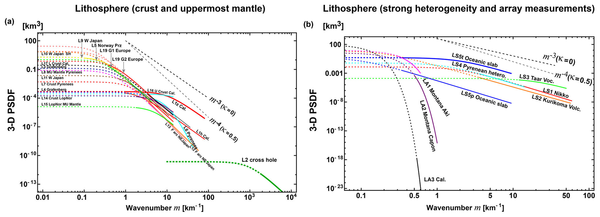
There have been measurements of velocity tomography at various scales, from which we can calculate the PSDF and then estimate von Kármán-type parameters. This method depends on the spatial resolution of the tomography result. Measurement L1 in Table 2 is calculated from the precise VP tomography result of the shallow crust, Los Angeles, California: the exponent of wavenumber is −3.08 (κ=0.04). Anisotropic randomness is also reported: az=0.1 and ah=0.5 km (see Eq. 3), we show those in Fig. 3a. Measurement M2 in Table 3 is evaluated from the 2-D PSDF of the VS tomography result of the upper mantle in a low wavenumber range. Although there is a resolution limit of the tomography method, the exponent of wavenumber is between −2 and −3, which means . We note that Fig. 8 of Mancinelli et al. (2016a) shows that the 1-D PSDF estimated from the VP tomography result in the upper mantle (Meschede and Romanowicz, 2015) covers that of MU2 (κ=0.05, ε=0.1, a=2000 km) for the wavenumber range from to 10−2 km−1.
Chevrot et al. (1998)Mancinelli et al. (2016a)Shearer and Earle (2004)Shearer and Earle (2004)Cormier (1999)Mancinelli et al. (2016b)Zhang et al. (2018)Margerin and Nolet (2003)Bentham et al. (2017)Table 3Reported von Kaŕmán parameters of the upper mantle and the lower mantle. A value in parentheses ( ) is a priori assumed in the measurement. When the estimated value is given by a range, a value in square brackets [ ] is used for plotting the PSDF. A label with an asterisk * is insufficient for plotting the PSDF.
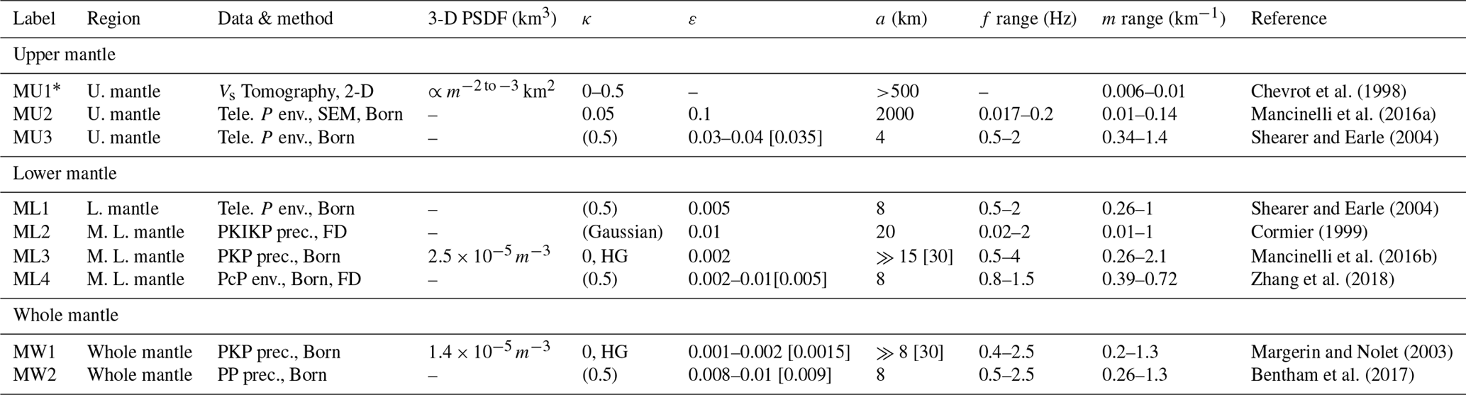
3.4 Array analysis of teleseismic P waves
Teleseismic P waves registered by a large aperture array were used for the evaluation of the 3-D PSDF of the lithosphere beneath the array: LA1 and LA2 of Table 2 in Montana and LA3 in southern California used amplitude and phase coherence analyses, where a Gaussian-type PSDF (Eq. 5b) was assumed because of mathematical simplicity. As shown in Fig. 3b, they drop very fast as wavenumber increases. Later Flatté and Wu (1988) developed the angular coherence analysis in addition to the above methods. Analyzing teleseismic P waves registered at NORSAR, they proposed an overlapping two-layer model LA4, which is composed of a band-limited flat spectrum from the surface to 200 km of depth and m−4 spectrum (κ=0.5, ε=0.01–0.04) for depths from 15 to 250 km. It means κ<0.5 and the decay of their PSDF is much smaller than that of Gaussian types (not shown in Fig. 3b).
3.5 Finite difference (FD) simulations
FD simulation is often used for the numerical simulation of waves in an inhomogeneous velocity structure. For the evaluation of average MS amplitude envelopes, we have to repeat simulations of the wave propagation through random media having the same PSDFs that are generated by using different random seeds. There are several measurements of statistical parameters using FD such as L9–L11 and ML4 in Tables 2 and 3. Measurement LS5 focused on the fact that the subducting oceanic plate is an efficient waveguide for high-frequency seismic waves: estimated anisotropic parameters are κ=0.5 and ε=0.02 with ap=10 km and at=0.5 km in the parallel and transverse directions, respectively. Note that ML2 supposes a Gaussian-type function.
3.6 Analyses of seismogram intensities (MS amplitude envelopes)
The RTT is essentially stochastic to directly synthesize the intensity (the average MS amplitude envelope) of a wavelet propagating through random media. There are two conventional methods on the basis of the RTT: one uses the Born approximation and the other uses the phase screen approximation based on the parabolic approximation when the wavenumber is larger than the corner. The former neglects the phase shift, but the latter correctly considers the phase shift.
3.6.1 Scalar wave scattering by a single obstacle
We here study the deterministic scattering of scalar waves by a single spherical obstacle (radius a=5 km and velocity anomaly ) embedded in a homogeneous medium (V0=4 km s−1) as a mathematical model. The Born approximation calculates spherically outgoing scattered waves putting the incident plane wave of wavenumber kc in the interaction term of the first-order perturbation equation. From the scattering amplitude we evaluate the total scattering cross section σ0 as a measure of scattering power of the obstacle. The resultant σ0 monotonously increases with frequency as shown by a blue line in Fig. 6. As the wavenumber increases (akc≫1), the phase shift increases as the incidence plane wave penetrates into the obstacle. Putting the phase modulated wave according to the parabolic approximation (the phase screen approximation) into the interaction term of the first-order perturbation equation, we calculate the scattering amplitude and then the total scattering cross section. This is the distorted-wave Born approximation with the phase screen approximation, which is also referred to as the eikonal approximation. This approximation predicts that σ0 (a red line in Fig. 6) saturates at high frequencies and converges to 2πa2, which is twice the geometrical section area of the obstacle as predicted by shadow scattering (e.g., Landau and Lifshitz, 2003, p. 519 and 543). We recognize that the conventional Born approximation is still accurate even for akc>1; however, it works well only for . We should use the distorted-wave Born approximation with the phase screen approximation for . The two approximations predict nearly the same σ0 value in the intermediate range. We note that 2εakc is the phase shift on the center line after passing the obstacle. Note that the phase screen approximation is not applicable for akc<1 since it is based on the parabolic approximation.
Interpreting ε and a as the RMS fractional fluctuation and the characteristic length of uniformly distributed random media, we may use the inequality or as a criterion of the Born approximation used in the RTT.
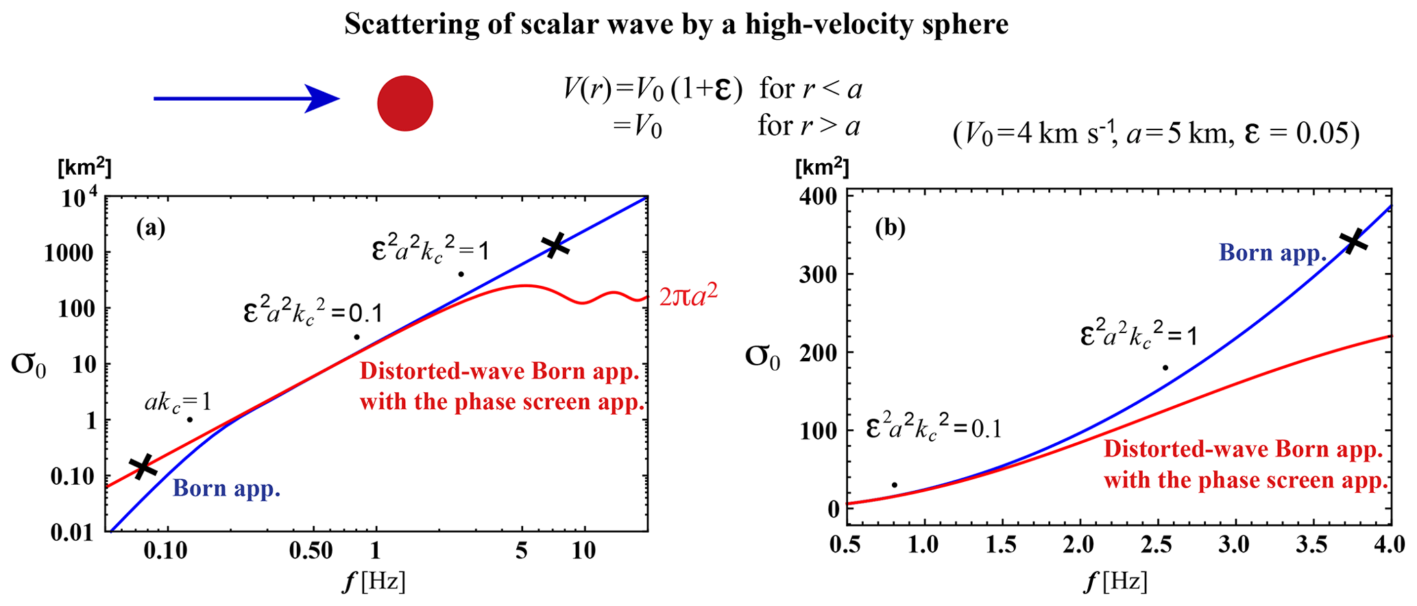
Figure 6Deterministic scattering of scalar waves by a high-velocity sphere. (a) Log–log plot of the total scattering cross section against frequency. (b) Semi-log plot for zoomed in graph. The Born approximation and the distorted-wave Born approximation with the phase screen approximation are drawn by blue and red lines, respectively.
3.6.2 RTT with the Born approximation
For uniformly distributed random media characterized by P(m), the Born approximation leads to the scattering coefficient at wavenumber kc into scattering angle ψ:
which is axially symmetric. The total scattering coefficient is
where . The integral kernel in the wavenumber space is given by
The upper bound of the integral is twice the wavenumber. As an example, Fig. 7 shows plots of P(m) (blue) vs. m, and gker(m) vs. m at 0.1 Hz (red) and 1 Hz (green) for the case of κ=0.5, ε=0.05, a=1 km, and V0=4 km s−1. As shown at the upper-right corner, the scattering pattern at 1 Hz (green) has a large lobe into the forward direction; however, it becomes isotropic as the frequency decreases. Dots on each gker curve show corresponding scattering angles.
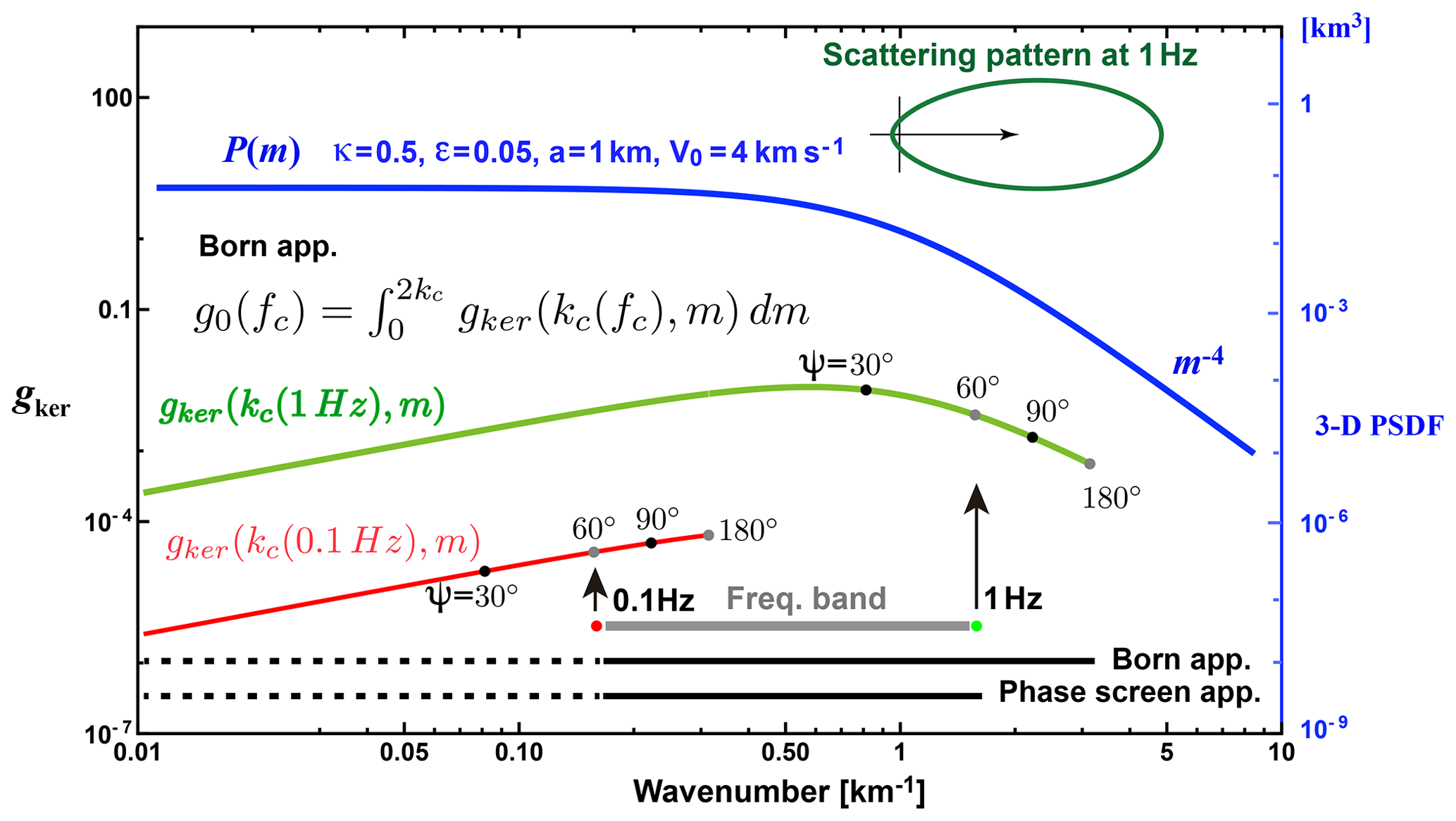
Figure 7Plot of P(m) (blue, right scale) and the spectral kernel of the scattering coefficient gker(kc(fc),m) at fc=0.1 Hz (red, left scale) and 1 Hz (green, left scale) according to the Born approximation. Scattering angles are marked by dots on each trace. For the case of the frequency band between 0.1 and 1 Hz, the phase screen approximation based on the parabolic approximation covers the wavenumber range from 0 to the upper bound (line at the bottom); however, the Born approximation covers the range from 0 to twice the upper bound (line next to the bottom). We also use these line styles in Figs. 3–5 and 9.
In the framework of the RTT, the Monte Carlo simulation is a simple method to stochastically synthesize the wavelet intensity time trace. A particle carrying unit intensity is shot randomly from a point source, and its trajectory is traced with the increment of time steps. The occurrence of scattering is stochastically tested by the inequality g0V0Δt> Random[0,1] at every time step of Δt, and is used as the probability of scattering into angle ψ. Note that Random[0,1] is a uniform random variable between 0 and 1. Since g0V0Δt is chosen to be small enough, scattering does not occur every time step but intermittently. As a simple example, Fig. 8a schematically illustrates the flowchart of the Monte Carlo simulation for the isotropic radiation from a point source in uniform random media. At lapse time t, dividing the number of particles n registered in a spherical shell of radius r and a thickness Δr by the total number of particles N and the shell volume 4πr2Δr, we calculate the intensity Green function G(r,t). The intensity time trace I(r,t) is calculated by the convolution of G(r,t) and the source intensity time function S(t) in the time domain. It is easy to introduce a layered structure of background velocity and intrinsic absorption into the simulation code.
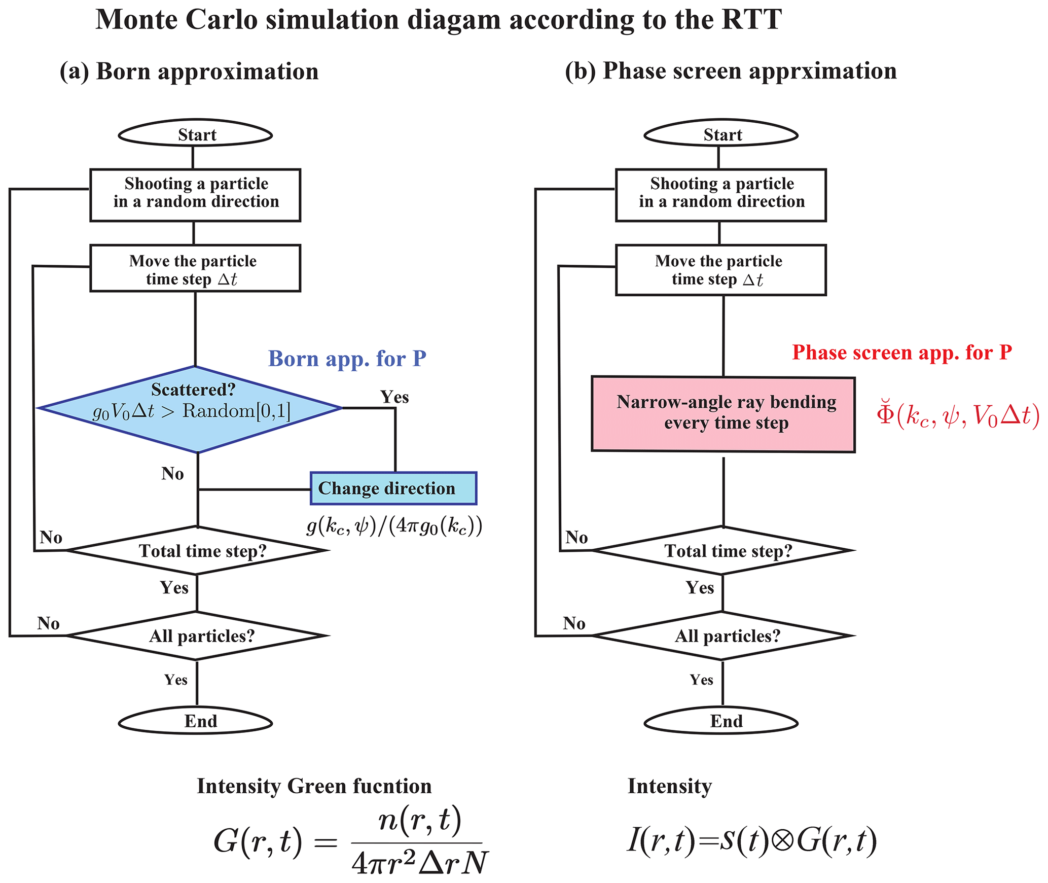
Figure 8Flowchart of the Monte Carlo simulation code according to the RTT for the scalar wavelet intensity in uniform random media. (a) RTT with the Born approximation. (b) RTT with the phase screen approximation.
The RTT for the scalar wave case can be extended to the elastic vector wave case by using Stokes parameters. There are four scattering modes: PP, PS, SS, and SP scatterings, and the S-wave scattering coefficients are not axially symmetric (see Sato et al., 2012, Fig. 4.7). Many papers (e.g., Shearer and Earle, 2004; Przybilla et al., 2009) suppose proportional relations and based on the empirical Birch's law, which reduce three fractional fluctuations into one (e.g., Sato et al., 2012, Eqs. 4.58 and 4.59).
The RTT with the Born approximation has been often used not only for the analyses of S coda envelopes but also for the whole seismogram envelope from the P onset via P coda through S wave until S coda (see Tables 2 and 3). This method has been often used not only for the analyses of regional seismograms propagating through the lithosphere but also for the analyses of teleseismic waves propagating through the mantle. This method is not only applied to direct P phase waves but also PcP and PKPprec phase waves and so on. In this review, we neglect intrinsic attenuation parameters a priori assumed or measured in each paper. For a given wavenumber range (kl,ku) (gray) in Fig. 7, each PSDF curve using this method in Figs. 3–5 and 9 is drawn by a dotted line for (0,kl) and a solid line for (kl,2ku) as the line next to the bottom of Fig. 7. As indicated by dots on the gker curves, the wavenumber interval of the solid line reflects wide-angle scattering and that of dotted line reflects narrow-angle scattering around the forward direction.
Most measurements of S waves in the lithosphere cover the wavenumber range up to 100 km−1. Measurement L2 analyzed cross-hole seismograms on the order of kHz by using 2-D RTT, of which the wavenumber range is as high as on the order of 1 m−1. Measurement MU2 for teleseismic P-wave envelopes at long periods in the upper mantle shows that the characteristic scale a=2000 km is much larger than those of MU3 and ML1 at short periods. Several measurements a priori suppose κ=0.5; however, most measurements show κ<0.5 except L6. Measurements ML3 and MW1 propose the HG type (see Eq. 4b) corresponding to κ=0 for the lower or whole mantle. We note that Mancinelli et al. (2016b) proposed an alternative model of 3-D PSDF in addition to ML3 (not shown in Fig. 4).
3.6.3 RTT with the phase screen approximation
When akc≫1, scattering mostly occurs within a narrow angle around the forward direction. At a large travel distance, the wavelet just after the onset is mostly composed of those waves. The phase screen approximation correctly calculates the phase shift modulation. For the incidence of a plane wave into the z direction, the mutual coherence function (MCF) of the phase shift modulated waves for an increment Δz is given by
The longitudinal integral of the ACF is
where x⊥ is the transverse coordinate vector and Sato et al. (2012, Eq. 9.60). Taking the Fourier transform of MCF Φ with respect to transverse coordinates, we have
Since , interpreting as the probability of ray-bending angle per increment Δz=V0Δt, we can stochastically synthesize the intensity by using the Monte Carlo simulation (e.g., Williamson, 1972; Takahashi et al., 2008; Saito et al., 2008). As a simple example, Fig. 8b schematically illustrates the flowchart of the RTT with the phase screen approximation for the isotropic radiation from a point source in uniform random media. Different from the Born approximation, narrow-angle ray bending occurs at every time step. The intensity Green function can be obtained in the same manner as the RTT with the Born approximation. This approximation synthesizes the intensity time trace having a delayed peak from the onset and a decaying tail of early coda at large travel distances. This approximation can not synthesize the late coda intensity since wide-angle scattering is neglected. The Markov approximation is known as a stochastic extension of the phase screen method for the two-frequency mutual coherence function (e.g., Saito et al., 2002). If we focus on the intensity time trace around the peak arrival, the Markov approximation and the RTT with the phase screen approximation show good coincidence (see Sato and Emoto, 2018, Fig. 8).
When this approximation is used, is a priori supposed. Most of this type of measurement reads the peak delay and the envelope width of each seismogram envelope. There is some merit to the fact that the peak delay measurement is rather insensitive to intrinsic absorption. In NE Japan, a κ value beneath a volcano LS2 is smaller than those in the fore-arc side L12 and L13. Note that narrow-angle scattering around the forward direction dominates in teleseismic wavelets even if the Born approximation is used for the analysis. Narrow-angle scattering is mostly produced by the PSDF in low wavenumbers compared with kc. For a given wavenumber range (kl,ku) (gray) in Fig. 7, each PSDF curve using this method in Fig. 3 is drawn by a dotted line for (0,kl) and a solid line for (kl,ku) as the bottom line of Fig. 7.
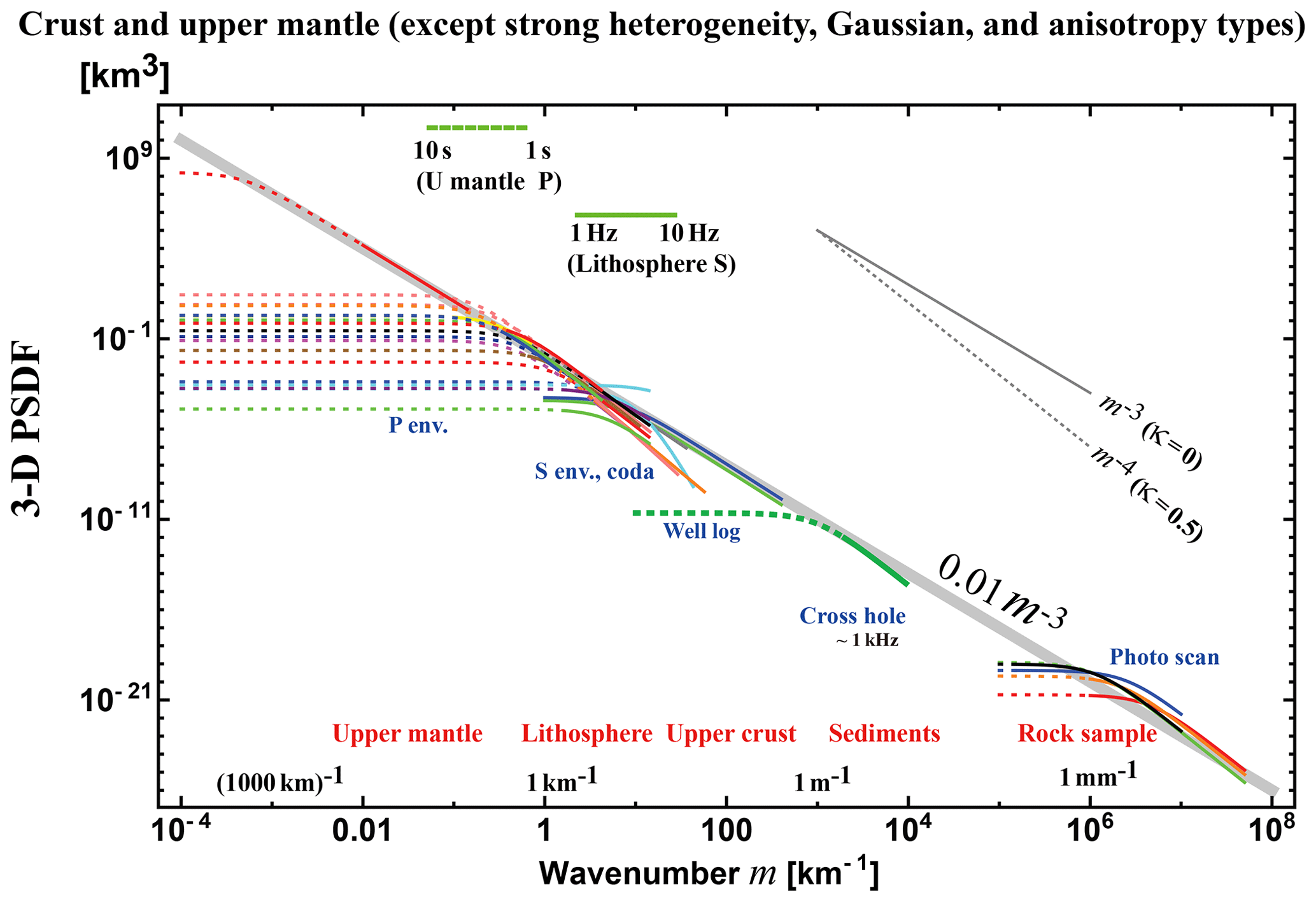
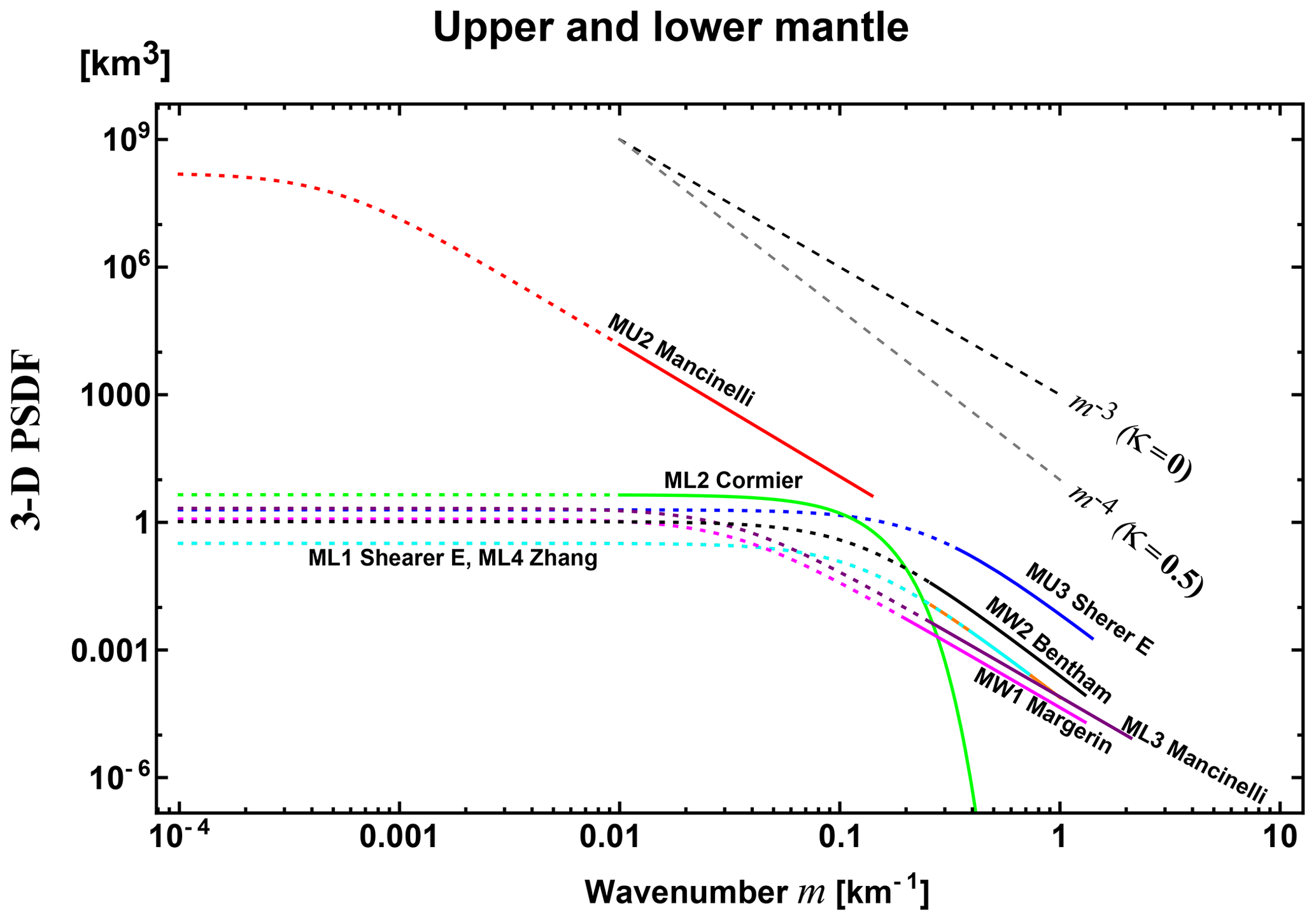
Figure 93-D PSDF vs. wavenumber for the crust and the upper mantle. Data of Gaussian-type, anisotropy type, strong heterogeneity, the lower mantle, and the whole mantle are excluded. The light-gray straight line visually fits to most spectral envelopes.
3.7 Characteristics of reported PSDFs
3.7.1 All the data
Some measurements a priori assumed κ=0.5; however, most of measurements report κ<0.5. In the mantle, κ is very small and close to zero, and a HG-type function is also proposed. The RMS fractional fluctuation ε is on the order of 0.1 for rock samples and well-log data, and in the range from 0.01 to 0.1 in the lithosphere and the upper mantle. Large values are reported for the shallow crust L16 and beneath a volcano LS3; however, smaller values are reported for the lower mantle. The characteristic scale a varies a lot depending on measurements. The corner wavenumber a−1 is not clearly seen in PSDFs of acoustic well logs. Some measurements report anisotropy: W3 of well-logs, L1 of velocity tomography in the shallow crust, and LS5 in the subducting oceanic slab. The characteristic length in the vertical direction is smaller than the horizontal direction in the shallow crust, and that in the transverse direction is smaller than that in the direction parallel to the subducting slab.
Plotting PSDFs against wavenumber is more informative for understanding the random heterogeneity compared with enumerating statistical parameter values. Figure 5 shows the plot of 3-D PSDF vs. wavenumber for all the data covering a wide wavenumber range (10−4–108 km−1). We recognize that the Gaussian type PSDFs show a very different behavior from others, which suggests the Gaussian-type assumption is inappropriate. PSDFs in the lower mantle take smaller values, and those for volcanoes and for the shallow crust take larger values than others.
3.7.2 Lithosphere and the upper mantle except strong heterogeneity, Gaussian, and anisotropy types
Eliminating data supposing a Gaussian-type data LA1–LA3, strong heterogeneity data LS1–LS4, anisotropy-type data L1 and LS5, and the lower mantle and the whole mantle data ML1–ML4 and MW1–MW2 from Fig. 5, we plot the rest of the data for the crust and the upper mantle in Fig. 9. Most ε values are in the range of 0.01–0.1, most κ values are less than or equal to 0.5 and many of them are close to 0, and the high wavenumber end of the power-law decay branch of each PSDF is not far from each corner wavenumber.
We draw a power-law decay line PSDF km3 (gray) visually fitting to most PSDF envelopes for a very wide range of wavenumbers (10−3–108 km−1). This line is not the average of PSDFs. This line looks like an extension of MU2 in the upper mantle into higher wavenumbers of the shallow crust.
4.1 Measurements
It will be necessary for us to measure the small-scale randomness of sedimentary rock samples. More measurements are necessary in the wavenumber range 103–105 km−1 since there are few measurements.
In most PSDF measurements, each power-law decay branch is short since the Born approximation senses the spectrum up to twice the wavenumber. It will be necessary to measure how each power-law decay branch varies with wavenumber increasing. It will be necessary to estimate the corner a−1 in each measurement with a wide wavenumber range covering, sufficiently large enough, both sides of the corner. The flat part, the low-wavenumber side of each PSDF drawn by a dotted line in figures is also important as the cause of narrow-angle scattering.
Although most measurements used in this review analyzed intrinsic attenuation, we did not enumerate them in this review since different assumptions were used in different measurements. It will be necessary for us to systematically measure the PSDF of random heterogeneity in conjunction with intrinsic attenuation.
We should note that there are large variations in δln VS∕δln VP and in the earth. Koper et al. (1999) estimated δln VS∕δln VP to be in the range 1.1–1.5 in the Tonga Slab. Romanowicz (2001) estimated δln VS∕δln VP to be larger than 2.5 in the lower mantle at larger length scales. Many measurements reported use ν=0.8 for the synthesis, which is appropriate for the shallow lithosphere. Parameter ν takes smaller values of 0.17 for volcanic-tuff (Shiomi et al., 1997) and 0.31–0.33 for sandstone and shale (Kenter et al., 2007). In the mantle, Karato (2008) estimated ν=0.23–0.42 for the S-wave velocity predicted from the temperature derivatives of seismic wave velocities and thermal expansion, and ν=0.15–0.23 including the influence of anelasticity. It will be necessary to introduce realistic δln VS∕δln VP and δln ρ∕δln VS in the synthesis.
Figure 9 summarizes reported PSDF measurements supposing isotropic randomness; however, there are measurements clearly showing anisotropic randomness such as W3 and L1 for the shallow crust and LS5 for the oceanic slab. Those may reflect the effect of gravity for the creation of anisotropy. It will be necessary for us to study how a wavelet propagates through anisotropic random heterogeneity of the earth medium (e.g., Margerin, 2006).
4.2 Mathematical theory
In Sect. 3.6.1, we mentioned that the conventional Born approximation is inapplicable and the phase screen approximation is useful when the phase shift becomes large as the wavenumber increases. In order to avoid the difficulty, taking the center wavenumber of a wavelet as a reference, Sato and Emoto (2018) proposed to divided the PSDF into two components (see also Sato, 2016; Sato and Emoto, 2017). They use the Born and phase-screen approximations to the short-scale (high wavenumber) and long-scale (low wavenumber) components, PS and PL, respectively, in the RTT in order to simultaneously explain the envelope broadening just after the onset and the excitation of late coda waves. Figure 10 illustrates the flowchart of their Monte Carlo simulation. Their spectrum division method looks like an implementation of the distorted-wave Born approximation in the RTT since it describes wide-angle scattering for the incidence of the phase-shift modulated wave. They successfully synthesized intensity time traces that explain FD simulation results for the case of akc=23.6 and . It would be interesting to see how this method may be extended to polarized elastic waves.
We note that some papers numerically show that the RTT with the Born approximation works well in some cases over the above limitation. Przybilla et al. (2006) synthesizes vector-wave intensity that fits to that of the FD simulation in 2-D, even for S waves of akc=58 and (see their Table 1) if the wandering effect is convolved as a result of the travel time fluctuation. Emoto and Sato (2018) show that the synthesized scalar intensity by the RTT with the Born approximation fits to that of the FD simulation in 3-D, even for the case of akc=23.6 and when the wandering effect is convolved. If the earth heterogeneity is represented by a power-law decay power spectrum for such a wide wavenumber range, which means that the corner wavenumber is very low, we should carefully examine the applicability of the Born approximation in the RTT.
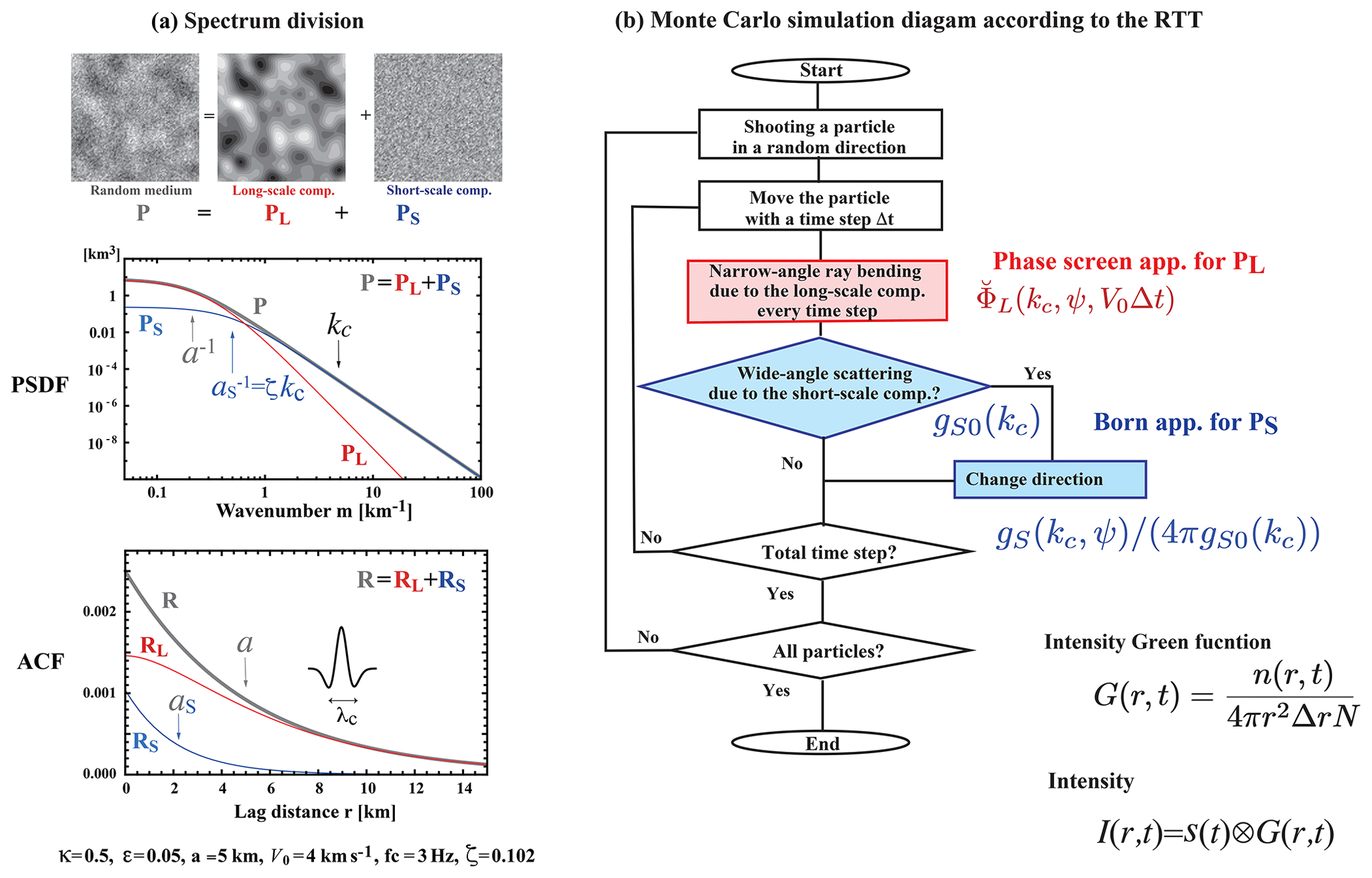
Figure 10Spectrum division method. (a) Division of P into two components, PS and PL, with respect to the center wavenumber of a wavelet kc as a reference, where ζ is a tuning parameter. (b) Flowchart of the Monte Carlo simulation according to the RTT with the spectrum division method. Modified from Sato and Emoto (2018).
Acoustic well-log and photo-scan methods faithfully measure the inhomogeneous elastic coefficients. The RTT used here supposes the scattering contribution of random inhomogeneity of elastic coefficients only; however, observed seismograms do not only reflect those but also the scattering contribution of pores and cracks distributed over the earth medium. It will be necessary for us to study their contribution in the intensity synthesis.
4.3 Power-law decay spectral envelope
In observation, we may take the power-law spectral envelope as a reference curve for studying the regional differences, especially in the power-law decay part of the PSDF. The characteristic length a seems to increase as the wavenumber of a wavelet decreases or as the dimension of measurement system becomes large. It reminds us that the characteristic scale of the slip distribution increases with increasing source dimension as Mai and Beroza (2002) analyzed finite-fault source inversion results (see their Fig. 12).
The power-law decay spectral envelope reminds us of the observed fractal nature of various kinds of surface topographies: Sayles and Thomas (1978a, b) show a 1-D PSDF for wavelengths 10−6–103 km although the power exponent varies from −1.07 to −3.03 for small segments; Brown and Scholz (1985) show a 1-D PSDF for the wavenumber range 10−6 to 0.1 µm−1, especially for the topography of natural rock surfaces and faults. We also note that the PSDF of the refractive index fluctuation of air obeys the Kolmogorov spectrum: 3-D PSDF , where . This spectrum is physically produced by the cascade in the turbulent flow of low viscosity air: the large eddies breaks up originating smaller eddies dissipating energy by viscosity. However, it may be difficult to apply this cascade model to the mantle since the viscosity of mantle fluid is thought to be high.
For igneous rocks such as granite, there are variations in composition of minerals and grain sizes, which depend on a variety of slow crystallization differentiations of basaltic magma. Random variations in acoustic well-log profiles reflect the complex sedimentation process during the geological history. Volcanism produces more heterogeneous structures composed of pyroclastic material and lava. For random heterogeneities in the mantle, we imagine complex mantle flow. Mancinelli et al. (2016a) referred to a marble cake mantle model (Allègre and Turcotte, 1986) containing heterogeneity mostly composed of basalt and harzburgite at many scales in the upper mantle in order to explain the power-law spectrum. Stixrude and Lithgow-Bertelloni (2007) proposed the velocity variation due to chemical and phase stability at different depths, which is a possible candidate especially for heterogeneity in the vertical direction. If we accept the power-law decay spectrum, we will have to study what kinds of geophysical mechanisms created such random medium spectra at different scales and in different geological environments in the solid earth.
4.4 Isotropic scattering coefficient
In advance of the measurements based on the RTT for anisotropic scattering presented here, there have been many measurements of the isotropic scattering coefficient giso in the world on the basis of the RTT with the isotropic scattering assumption (e.g., Sato et al., 2012; Yoshimoto and Jin, 2008). The isotropic scattering model is mathematically tractable, and the multiple lapse-time window analysis (Fehler et al., 1992; Hoshiba, 1993) has often been used for practical analyses. This method essentially estimates giso from the ratio of late coda excitation to the radiated energy irrespective of the envelope broadening. Recent measurements show that giso decreases with depth (e.g., Rachman and Chung, 2016; Badi et al., 2009). It will be interesting to plot the frequency dependence of reported giso for a wide range of frequencies and to study the relation with the obtained power spectral envelope shown in Fig. 9.
Recent seismological observations focusing on the collapse of an impulsive wavelet revealed the existence of small-scale random heterogeneities in the earth medium. The RTT has often been used for the study of the propagation of wavelet intensities, the MS amplitude envelopes. For the statistical characterization of the PSDF of random velocity inhomogeneities in a 3-D space, we have used von Kármán type functions with three parameters: the RMS fractional velocity fluctuation ε, the characteristic length a, and the order κ of the modified Bessel function of the second kind. This model leads to the power-law decay of PSDF at wavenumber m higher than the corner at a−1. We have compiled reported statistical parameters of the lithosphere and the mantle based on various types of measurements for a wide range of wavenumbers: photo-scan data of rock samples, acoustic well-log data, and envelope analyses of cross-hole experiment seismograms, regional seismograms, and teleseismic waves based on the RTT. Reported κ values are distributed between 0 and 0.5 (PSDF ), where many of them are close to 0 (PSDF ). Reported ε values are on the order of 0.01–0.1 in the crust and the upper mantle, where smaller values in the lower mantle and higher values beneath volcanoes. Reported a values distribute very widely; however, each one seems to be restricted by the dimension of the measurement system or the sample length. In order to grasp the spectral characteristics, eliminating strong heterogeneity data and the lower mantle data, we have plotted all the reported PSDFs in the crust and the upper mantle against wavenumber m for a wide range (10−3–108 km−1). We find that the envelope of those PSDFs is well approximated by a power-law decay curve 0.01 m−3 km3. Multiple plots of PSDFs and the power-law decay spectral envelope obtained require us to do the following. In theory, it will be necessary to examine whether the Born approximation is reliable or not if the wavenumber increases much larger than the corner; in observation, we will have to more carefully examine the behavior of each PSDF on both sides of the corner. If we accept the power-law decay spectral envelope, it suggests that the earth-medium randomness has a broad spectrum. We may consider the obtained power-law decay spectral envelope as a reference for studying the regional differences. It is interesting to study what kinds of geophysical processes created the power-law spectral envelope at different scales and in different geological environments of the solid earth medium.
All the data for this review work are listed in Tables 1–3, where all the references are given.
The author HS reviewed reported measurement of statistical parameters characterizing the random heterogeneities in the earth.
The author declares that they have no conflict of interest.
This paper is a part of the Beno Gutenberg medal lecture at the 2018 EGU assembly held in
Vienna. The author is grateful to the seismology section of EGU for giving him an
opportunity for reviewing measurements of random heterogeneities in the solid earth and
various theoretical approaches. The author expresses sincere thanks to his colleagues and
ex-graduate students who enthusiastically collaborated with him in studying seismic wave
scattering in random media. The author acknowledges reviewers, Vernon Cormier, Michael
Korn, and Ludovic Margerin and editor Tarje Nissen-Meyer for their helpful comments and
suggestions.
Edited by: Tarje Nissen-Meyer
Reviewed by: Ludovic Margerin, Michael Korn, and Vernon Cormier
Aki, K.: Scattering of P waves under the Montana LASA, J. Geophys. Res., 78, 1334–1346, https://doi.org/10.1029/JB078i008p01334, 1973. a
Aki, K. and Chouet, B.: Origin of coda waves: Source, attenuation and scattering effects, J. Geophys. Res., 80, 3322–3342, 1975. a, b
Allègre, C. J. and Turcotte, D. L.: Implications of a two-component marble-cake mantle, Nature, 323, 123–127, 1986. a
Badi, G., Pezzo, E. D., Ibanez, J. M., Bianco, F., Sabbione, N., and Araujo, M.: Depth dependent seismic scattering attenuation in the Nuevo Cuyo region (southern central Andes), Geophys. Res. Lett., 36, L24307, https://doi.org/10.1029/2009GL041081, 2009. a
Bentham, H., Rost, S., and Thorne, M.: Fine-scale structure of the mid-mantle characterised by global stacks of PP precursors, Earth Planet. Sci. Lett., 472, 164–173, 2017. a
Brown, S. R. and Scholz, C. H.: Broad bandwidth study of the topography of natural rock surfaces, J. Geophys. Res.-Sol. Ea., 90, 12575–12582, 1985. a
Calvet, M. and Margerin, L.: Lapse-Time Dependence of Coda Q: Anisotropic Multiple-Scattering Models and Application to the Pyrenees, B. Seismol. Soc. Am., 103, 1993–2010, 2013. a
Capon, J.: Characterization of crust and upper mantle structure under LASA as a random medium, B. Seismol. Soc. Am., 64, 235–266, 1974. a
Carcolé, E. and Sato, H.: Spatial distribution of scattering loss and intrinsic absorption of short-period S waves in the lithosphere of Japan on the basis of the Multiple Lapse Time Window Analysis of Hi-net data, Geophys. J. Int., 180, 268–290, https://doi.org/10.1111/j.1365-246X.2009.04394.x, 2010. a
Chernov, L. A.: Wave Propagation in a Random Medium (Engl. trans. by R. A. Silverman), McGraw-Hill, New York, 1960. a
Chevrot, S., Montagner, J., and Snieder, R.: The spectrum of tomographic earth models, Geophys. J. Int., 133, 783–788, 1998. a
Cormier, V. F.: Anisotropy of heterogeneity scale lengths in the lower mantle from PKIKP precursors, Geophys. J. Int., 136, 373–384, 1999. a
da Silva, J. J. A., Poliannikov, O. V., Fehler, M., and Turpening, R.: Modeling scattering and intrinsic attenuation of cross-well seismic data in the Michigan Basin, Geophysics, 83, WC15–WC27, 2018. a, b
Dziewonski, A. and Anderson, D.: Preliminary Reference Earth Model (PREM), Phys. Earth Planet In., 25, 297–356, 1981. a
Emoto, K. and Sato, H.: Statistical characteristics of scattered waves in 3-D random media: Comparison of the finite difference simulation and statistical methods, Preprint, Geophys. J. Int., 215, 585–599, https://doi.org/10.1093/gji/ggy298, 2018. a
Emoto, K., Saito, T., and Shiomi, K.: Statistical parameters of random heterogeneity estimated by analysing coda waves based on finite difference method, Geophys. J. Int., 211, 1575–1584, 2017. a
Eulenfeld, T. and Wegler, U.: Crustal intrinsic and scattering attenuation of high-frequency shear waves in the contiguous United States, J. Geophys. Res.-Sol. Ea., 122, 4676–4690, 2017. a
Fehler, M., Hoshiba, M., Sato, H., and Obara, K.: Separation of scattering and intrinsic attenuation for the Kanto-Tokai region, Japan, using measurements of S-wave energy versus hypocentral distance, Geophys. J. Int., 108, 787–800, https://doi.org/10.1111/j.1365-246X.1992.tb03470.x, 1992. a
Flatté, S. M. and Wu, R. S.: Small-scale structure in the lithosphere and asthenosphere deduced from arrival time and amplitude fluctuations at NORSAR, J. Geophys. Res., 93, 6601–6614, https://doi.org/10.1029/JB093iB06p06601, 1988. a, b
Fukushima, Y., Nishizawa, H., Sato, H., and Ohtake, M.: Laboratory study on scattering characteristics of shear waves in rock samples, B. Seismol. Soc. Am., 93, 253–263, https://doi.org/10.1785/0120020074, 2003. a, b, c, d
Furumura, T. and Kennett, B. L. N.: Subduction zone guided waves and the heterogeneity structure of the subducted plate: Intensity anomalies in northern Japan, J. Geophys. Res., 110, B10302, https://doi.org/10.1029/2004JB003486, 2005. a
Gaebler, P. J., Sens-Schönfelder, C., and Korn, M.: The influence of crustal scattering on translational and rotational motions in regional and teleseismic coda waves, Geophys. J. Int., 201, 355–371, 2015. a
Gusev, A. A. and Abubakirov, I. R.: Monte-Carlo simulation of record envelope of a near earthquake, Phys. Earth Planet. In., 49, 30–36, https://doi.org/10.1016/0031-9201(87)90130-0, 1987. a
Henyey, L. G. and Greenstein, J. L.: Diffuse radiation in the galaxy, Astrophys. J., 93, 70–83, 1941. a
Hock, S., Korn, M., Ritter, J. R. R., and Rothert, E.: Mapping random lithospheric heterogeneities in northern and central Europe, Geophys. J. Int., 157, 251–264, https://doi.org/10.1111/j.1365-246X.2004.02191.x, 2004. a, b, c
Holliger, K.: Upper-crustal seismic velocity heterogeneity as derived from a variety of P-wave sonic logs, Geophys. J. Int., 125, 813–829, https://doi.org/10.1111/j.1365-246X.1996.tb06025.x, 1996. a, b
Hoshiba, M.: Separation of scattering attenuation and intrinsic absorption in Japan using the multiple lapse time window analysis of full seismogram envelope, J. Geophys. Res., 98, 15809–15824, https://doi.org/10.1029/93JB00347, 1993. a
Hoshiba, M., Sato, H., and Fehler, M.: Numerical basis of the separation of scattering and intrinsic absorption from full seismogram envelope – A Monte-Carlo simulation of multiple isotropic scattering, Pap. Meteorol. Geophys., 42, 65–91, 1991. a
Jing, Y., Zeng, Y., and Lin, G.: High-Frequency Seismogram Envelope Inversion Using a Multiple Nonisotropic Scattering Model: Application to Aftershocks of the 2008 Wells Earthquake, B. Seismol. Soc. Am., 104, 823–839, 2014. a
Karato, S.: Deformation of earth materials: an introduction to the rheology of solid earth, Cambridge University Press, 2008. a
Kenter, J., Braaksma, H., Verwer, K., and van Lanen, X.: Acoustic behavior of sedimentary rocks: Geologic properties versus Poisson's ratios, The Leading Edge, 26, 436–444, 2007. a
Kobayashi, M., Takemura, S., and Yoshimoto, K.: Frequency and distance changes in the apparent P-wave radiation pattern: effects of seismic wave scattering in the crust inferred from dense seismic observations and numerical simulations, Geophys. J. Int., 202, 1895–1907, 2015. a
Koper, K. D., Wiens, D. A., Dorman, L., Hildebrand, J., and Webb, S.: Constraints on the origin of slab and mantle wedge anomalies in Tonga from the ratio of S to P velocities, J. Geophys. Res.-Sol. Ea., 104, 15089–15104, 1999. a
Korn, M.: Determination of site-dependent scattering Q from P-wave coda analysis with an energy-flux model, Geophys. J. Int., 113, 54–72, https://doi.org/10.1111/j.1365-246X.1993.tb02528.x, 1993. a
Kubanza, M., Nishimura, T., and Sato, H.: Evaluation of strength of heterogeneity in the lithosphere from peak amplitude analyses of teleseismic short-period vector P waves, Geophys. J. Int., 171, 390–398, https://doi.org/10.1111/j.1365-246X.2007.03544.x, 2007. a
Landau, L. and Lifshitz, E.: Quantum Mechanics, 3rd Edn., (Englidh translation by J. B. Sykes and J. S. Bell), Butterworth-Heinemann, 2003. a
Mai, P. M. and Beroza, G. C.: A spatial random field model to characterize complexity in earthquake slip, J. Geophys. Res.-Sol. Ea., 107, 1–10, 2002. a
Mancinelli, N., Shearer, P., and Liu, Q.: Constraints on the heterogeneity spectrum of Earth's upper mantle, J. Geophys. Res.-Sol. Ea., 121, 3703–3721, 2016a. a, b, c
Mancinelli, N., Shearer, P., and Thomas, C.: On the frequency dependence and spatial coherence of PKP precursor amplitudes, J. Geophys. Res.-Sol. Ea., 121, 1873–1889, 2016b. a, b
Margerin, L.: Introduction to radiative transfer of seismic waves, in: Seismic Earth: Array Analysis of Broadband Seismograms, edited by: Levander, A. and Nolet, G., Geophysical Monograph-American Geophysical Union, 157, 229–252, 2005. a
Margerin, L.: Attenuation, transport and diffusion of scalar waves in textured random media, Tectonophysics, 416, 229–244, 2006. a
Margerin, L. and Nolet, G.: Multiple scattering of high-frequency seismic waves in the deep Earth: PKP precursor analysis and inversion for mantle granularity, J. Geophys. Res., 108, 2514, https://doi.org/10.1029/2003JB002455, 2003. a
Margerin, L., Campillo, M., and Tiggelen, B. V.: Monte Carlo simulation of multiple scattering of elastic waves, J. Geophys. Res., 105, 7873–7893, https://doi.org/10.1029/1999JB900359, 2000. a
Meschede, M. and Romanowicz, B.: Lateral heterogeneity scales in regional and global upper mantle shear velocity models, Geophys. J. Int., 200, 1076–1093, 2015. a
Morioka, H., Kumagai, H., and Maeda, T.: Theoretical basis of the amplitude source location method for volcano-seismic signals, J. Geophys. Res.-Sol. Ea., 122, https://doi.org/10.1002/2017JB013997, 2017. a
Nakata, N. and Beroza, G. C.: Stochastic characterization of mesoscale seismic velocity heterogeneity in Long Beach, California, Geophys. J. Int., 203, 2049–2054, 2015. a, b
Petukhin, A. and Gusev, A.: The duration-distance relationship and average envelope shapes of small Kamchatka earthquakes, Pure Appl. Geophys., 160, 1717–1743, https://doi.org/10.1007/s00024-003-2373-5, 2003. a
Powell, C. A. and Meltzer, A. S.: Scattering of P-waves beneath SCARLET in southern California, Geophys. Res. Lett., 11, 481–484, https://doi.org/10.1029/GL011i005p00481, 1984. a
Przybilla, J., Korn, M., and Wegler, U.: Radiative transfer of elastic waves versus finite difference simulations in two-dimensional random media, J. Geophys. Res., 111, B04305, https://doi.org/10.1029/2005JB003952, 2006. a
Przybilla, J., Wegler, U., and Korn, M.: Estimation of crustal scattering parameters with elastic radiative transfer theory, Geophys. J. Int., 178, 1105–1111, https://doi.org/10.1111/j.1365-246X.2009.04204.x, 2009. a, b, c
Rachman, A. N. and Chung, T. W.: Depth-dependent crustal scattering attenuation revealed using single or few events in South Korea, B. Seismol. Soc. Am., 106, 1499–1508, 2016. a
Romanowicz, B.: Can we resolve 3D density heterogeneity in the lower mantle?, Geophys. Res. Lett., 28, 1107–1110, 2001. a
Rost, S., Thorne, M. S., and Garnero, E. J.: Imaging global seismic phase arrivals by stacking array processed short-period data, Seismol. Res. Lett., 77, 697–707, 2006. a
Rothert, E. and Ritter, J. R.: Small-scale heterogeneities below the Gräfenberg array, Germany from seismic wavefield fluctuations of Hindu Kush events, Geophys. J. Int., 140, 175–184, 2000. a
Saito, T., Sato, H., and Ohtake, M.: Envelope broadening of spherically outgoing waves in three-dimensional random media having power-law spectra, J. Geophys. Res., 107, 1–15, https://doi.org/10.1029/2001JB000264, 2002. a, b
Saito, T., Sato, H., Ohtake, M., and Obara, K.: Unified explanation of envelope broadening and maximum-amplitude decay of high-frequency seismograms based on the envelope simulation using the Markov approximation: Forearc side of the volcanic front in northeastern Honshu, Japan, J. Geophys. Res., 110, B01304, https://doi.org/10.1029/2004JB003225, 2005. a
Saito, T., Sato, H., and Takahashi, T.: Direct simulation methods for scalar-wave envelopes in two-dimensional layered random media based on the small-angle scattering approximation, Commun. Comput. Phys, 3, 63–84, 2008. a
Sanborn, C. J., Cormier, V. F., and Fitzpatrick, M.: Combined effects of deterministic and statistical structure on high-frequency regional seismograms, Geophys. J. Int., 210, 1143–1159, https://doi.org/10.1093/gji/ggx219, 2017. a, b, c
Sato, H.: Energy propagation including scattering effects: Single isotropic scattering approximation, J. Phys. Earth, 25, 27–41, 1977a. a
Sato, H.: Attenuation and envelope formation of three-component seismograms of small local earthquakes in randomly inhomogeneous lithosphere, J. Geophys. Res., 89, 1221–1241, https://doi.org/10.1029/JB089iB02p01221, 1984. a
Sato, H.: Broadening of seismogram envelopes in the randomly inhomogeneous lithosphere based on the parabolic approximation: Southeastern Honshu, Japan, J. Geophys. Res., 94, 17735–17747, https://doi.org/10.1029/JB094iB12p17735, 1989. a
Sato, H.: Envelope broadening and scattering attenuation of a scalar wavelet in random media having power-law spectra, Geophys. J. Int., 204, 386–398, https://doi.org/10.1093/gji/ggv442, 2016. a
Sato, H. and Emoto, K.: Synthesis of a scalar wavelet intensity propagating through von Kármán-type random media: joint use of the radiative transfer equation with the Born approximation and the Markov approximation, Geophys. J. Int., 211, 512–527, https://doi.org/10.1093/gji/ggx318, 2017. a
Sato, H. and Emoto, K.: Synthesis of a scalar wavelet intensity propagating through von Kármán-type random media: Radiative transfer theory using the Born and phase-screen approximations, Geophys. J. Int., 215, 909–923, 2018. a, b, c
Sato, H., Fehler, M. C., and Maeda, T.: Seismic wave propagation and scattering in the heterogeneous earth, 2nd Edn., Springer, 2012. a, b, c, d, e
Sayles, R. S. and Thomas, T. R.: Surface topography as a non-stationary random process, Nature, 271, 431–434, 1978a. a
Sayles, R. S. and Thomas, T. R.: Reply to “Topography of random surfaces”, Nature, 273, 573 pp., 1978b. a
Sens-Schönfelder, C., Margerin, L., and Campillo, M.: Laterally heterogeneous scattering explains Lg blockage in the Pyrenees, J. Geophys. Res., 114, B07309, https://doi.org/10.1029/2008JB006107, 2009. a, b, c
Shearer, P. M. and Earle, P. S.: The global short-period wavefield modelled with a Monte Carlo seismic phonon method, Geophys. J. Int., 158, 1103–1117, https://doi.org/10.1111/j.1365-246X.2004.02378.x, 2004. a, b, c, d
Shiomi, K., Sato, H., and Ohtake, M.: Broad-band power-law spectra of well-log data in Japan, Geophys. J. Int., 130, 57–64, https://doi.org/10.1111/j.1365-246X.1997.tb00987.x, 1997. a, b, c, d
Sivaji, C., Nishizawa, O., Kitagawa, G., and Fukushima, Y.: A physical-model study of the statistics of seismic waveform fluctuations in random heterogeneous media, Geophys. J. Int., 148, 575–595, https://doi.org/10.1046/j.1365-246x.2002.01606.x, 2002. a, b, c, d
Spetzler, J., Sivaji, C., Nishizawa, O., and Fukushima, Y.: A test of ray theory and scattering theory based on a laboratory experiment using ultrasonic waves and numerical simulation by finite-difference method, Geophys. J. Int., 148, 165–178, 2002. a
Stixrude, L. and Lithgow-Bertelloni, C.: Influence of phase transformations on lateral heterogeneity and dynamics in Earth's mantle, Earth Planet. Sci. Lett., 263, 45–55, 2007. a
Takahashi, T., Sato, H., and Nishimura, T.: Recursive formula for the peak delay time with travel distance in von Karman type non-uniform random media on the basis of the Markov approximation, Geophys. J. Int., 173, 534–545, https://doi.org/10.1111/j.1365-246X.2008.03739.x, 2008. a
Takahashi, T., Sato, H., Nishimura, T., and Obara, K.: Tomographic inversion of the peak delay times to reveal random velocity fluctuations in the lithosphere: method and application to northeastern Japan, Geophys. J. Int., 178, 1437–1455, https://doi.org/10.1111/j.1365-246X.2009.04227.x, 2009. a, b, c
Takemura, S., Furumura, T., and Saito, T.: Distortion of the apparent S-wave radiation pattern in the high-frequency wavefield: Tottori-Ken Seibu, Japan, earthquake of 2000, Geophys. J. Int., 178, 950–961, https://doi.org/10.1111/j.1365-246X.2009.04210.x, 2009. a
Wang, W. and Shearer, P.: Using direct and coda wave envelopes to resolve the scattering and intrinsic attenuation structure of Southern California, J. Geophys. Res.-Sol. Ea., 122, 7236–7251, 2017. a, b
Williamson, I. P.: Pulse broadening due to multiple scattering in the interstellar medium, Mon. Not. R. Astron. Soc., 157, 55–71, 1972. a
Wu, R. S., Xu, Z., and Li, X. P.: Heterogeneity spectrum and scale-anisotropy in the upper crust revealed by the German Continental Deep-Drilling (KTB) holes, Geophys. Res. Lett., 21, 911–914, https://doi.org/10.1029/94GL00772, 1994. a, b, c
Yoshimoto, K.: Monte-Carlo simulation of seismogram envelope in scattering media, J. Geophys. Res., 105, 6153–6161, https://doi.org/10.1029/1999JB900437, 2000. a
Yoshimoto, K. and Jin, A.: Coda Energy Distribution and Attenuation, in: Earth Heterogeneity and Scattering Effects on Seismic Waves, edited by: Sato, H. and Fehler, M. C., Advances in Geophysics (Series Ed. R. Dmowska), chap. 10, Academic Press, Vol. 50, 265–300, 2008. a, b
Yoshimoto, K., Sato, H., and Ohtake, M.: Three-component seismogram envelope synthesis in randomly inhomogeneous semi-infinite media based on the single scattering approximation, Phys. Earth Planet. In., 104, 37–61, https://doi.org/10.1016/S0031-9201(97)00061-7, 1997b. a
Zeng, Y.: Modeling of High-Frequency Seismic-Wave Scattering and Propagation Using Radiative Transfer Theory, B. Seismol. Soc. Am., 107, 2948–2962, 2017. a
Zhang, B., Ni, S., Sun, D., Shen, Z., Jackson, J. M., and Wu, W.: Constraints on small-scale heterogeneity in the lowermost mantle from observations of near podal PcP precursors, Earth Planet. Sci. Lett., 489, 267–276, 2018. a